CS180 Final Project: Neural Radiance Fields

Part 1: Fit a Neural Field to a 2D Image

In 2D space, there's no concept of radiance and volume rendering. This just means that a 2D Neural Field maps every pixel maps to an RBG color for that point. This means that a 2D Neural Field just outputs the same exact image as the input image. A big part of the network trained is a the Positional Encoder layer. Positional Encoder (PE) is a technique to help neural networks better handle continuous input values by encoding them into higher dimensional space using sine and cosine functions. I used L = 10 as mentioned in the project spec.

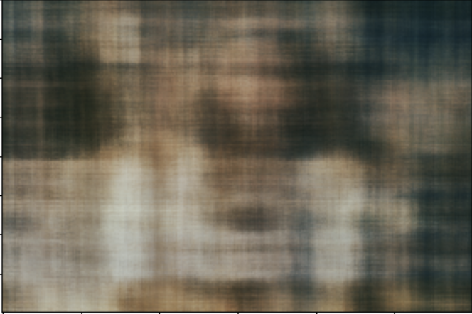
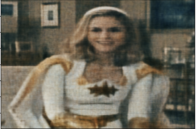
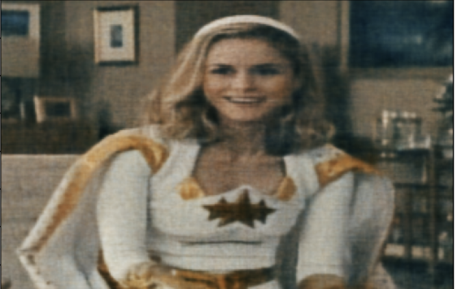
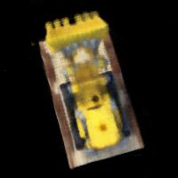
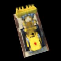
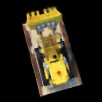
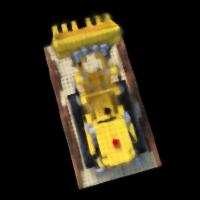
For the dataset, I created a class that creates training pairs of (pixel coordinates, colors) from an image. It randomly samples pixel positions and gets the corresponding RGB values. Both the coordinates and colors are normalized. I used the MSE loss, and reconstruct the PSNR using the MSE at each iteration. Here are the progressive results. With the last image being the final output after all the iterations. My architecture is the same as the one in the project spec. I used 3k iterations along with 10k batch size.

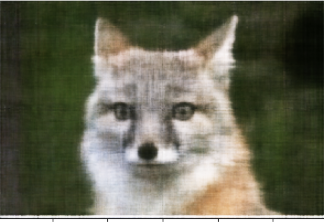
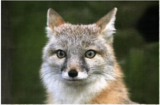
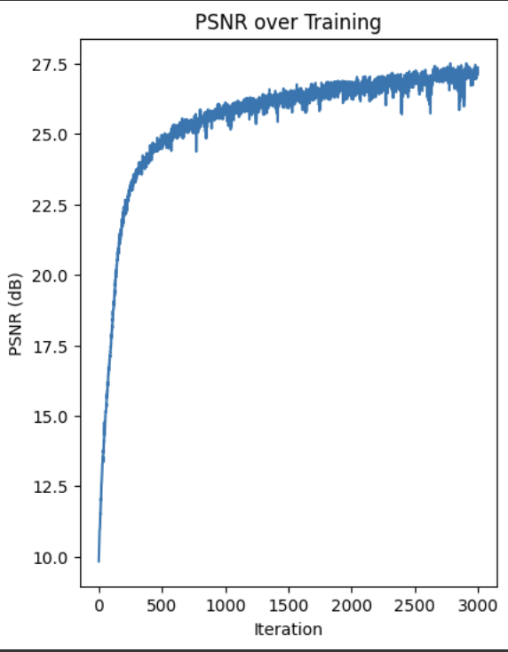
Here is the PSNR curve for the fox image.

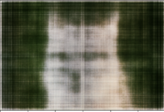
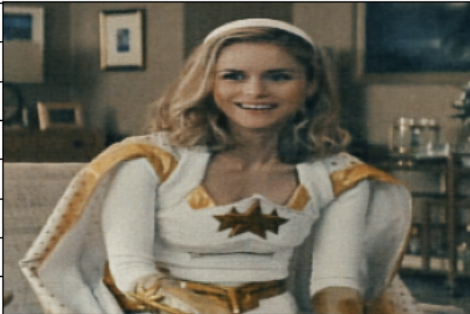
Here is the iterative results for my own image.

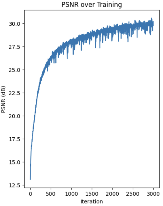
Here is the PSNR curve for my own image.

Part 2.1

A big part of this NeRF thing is being able to work with the camera parameters and transform between different coordinate systems. We need to be able to figure out where the rays are coming from and where they're pointing. That's crucial for accurately sampling the points along those rays. This section of the code sets up all the core geometric and coordinate system stuff we need to make that work. K is the intrinsic matrix, which is a 3x3 matrix representing all the internal camera settings, like the focal length and where the center of the image is. It's how we convert those 2D pixel coordinates into 3D points in the camera's coordinate system. Camera-to-World takes a 3D point in the camera coordinate system and transforms it into the world coordinate system using the c2w transformation matrix. I added a homoegnous dimension to make this work. Pixel-to-Camera takes a 2D pixel coordinate and a depth value to compute the corresponding 3D point in the camera coordinate system. I use the inverse of K to do this. Pixel-to-ray takes in 2D pixel coordinate and computes the ray origin and direction in the world coordinate system. The ray origin is the translation component of the camera-to-world transformation matrix. To get the direction of the ray, I converted 2D pixel coordinates to 3D points in the camera coordinate system then to world coordinate system and subtracted the ray origin. I also normalized the ray direction to have normal length.

Part 2.2

Now that the core geometry is taken care of, we are ready to sample. The RaysData class is responsible for managing the input data for the NeRF model. The sample_rays method returns the ray origins, ray directions, and the corresponding pixel values This data is crucial for training the NeRF model, as it provides the necessary information to learn the mapping between the 3D scene and the 2D images. It selects B images from the available training images, generates random 2D pixel coordinates within the dimensions of the training images, then it calls the pixel_to_ray function. I also utilized a helper function to sample points along the given rays, which just generates a set of sample points along the rays.

Part 2.3

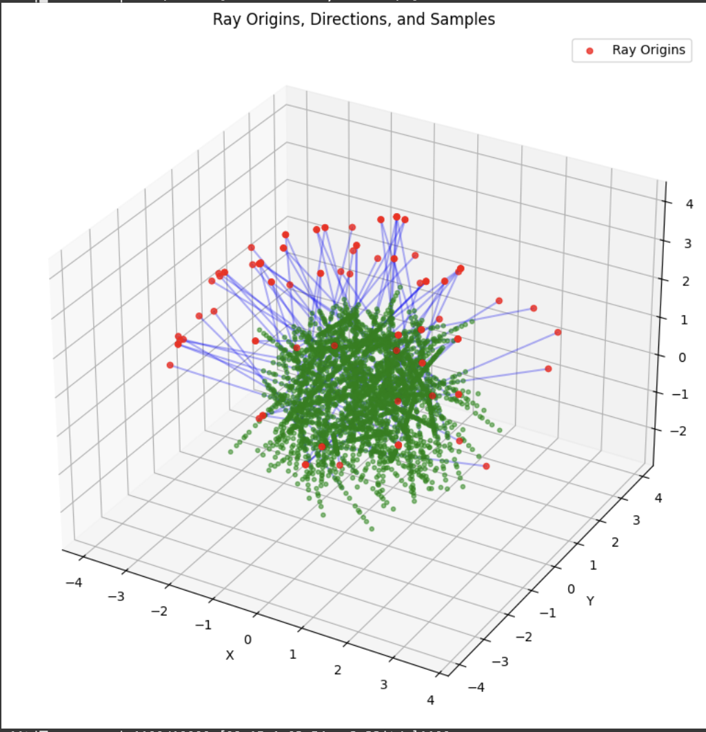
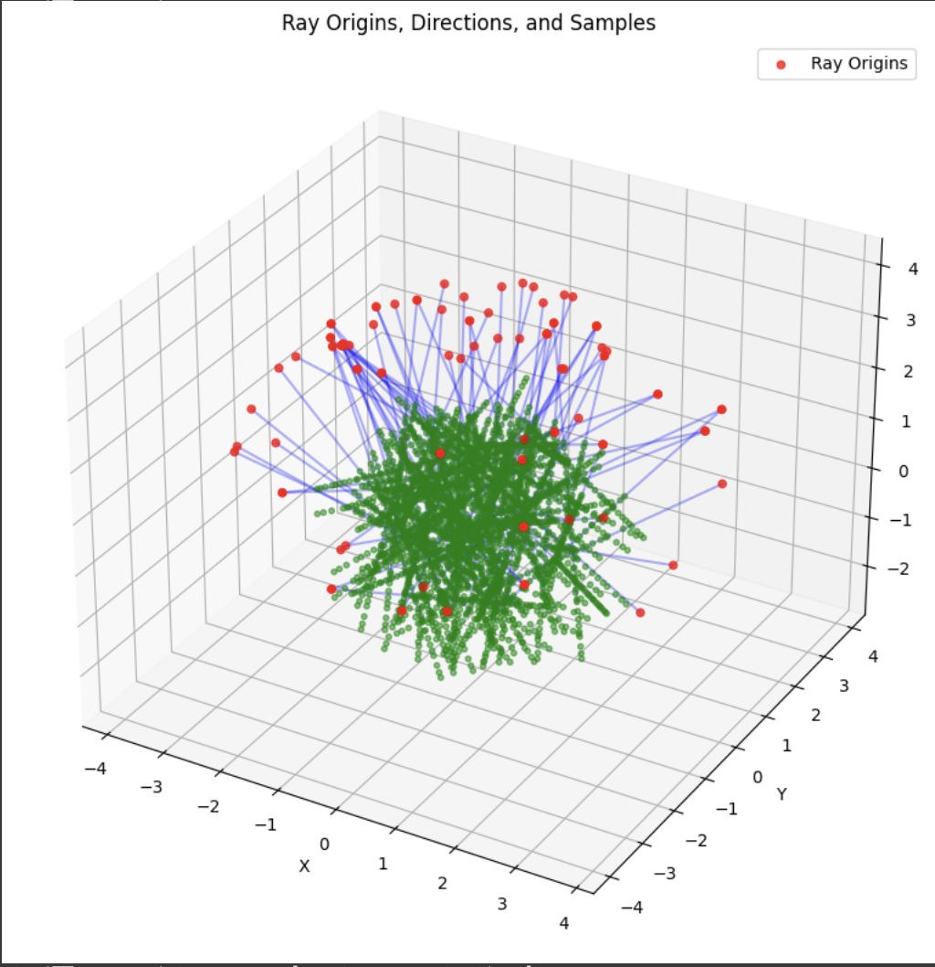
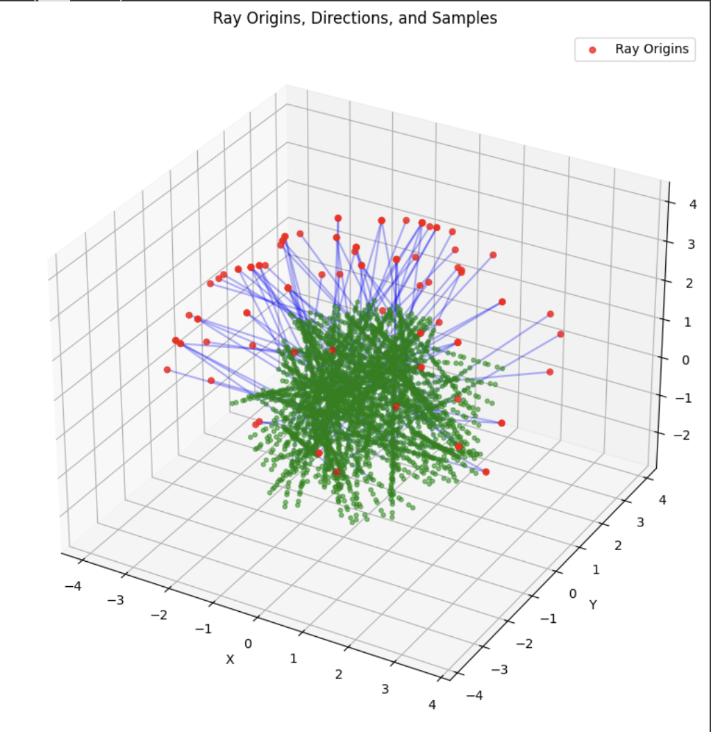
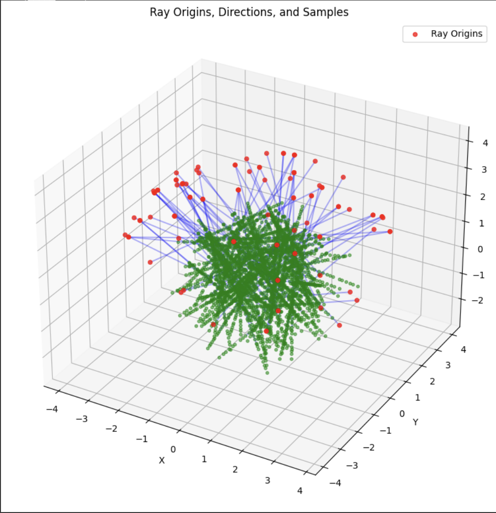
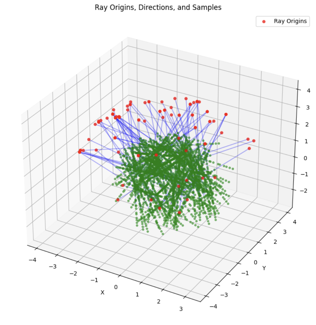
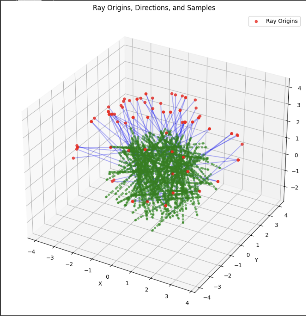
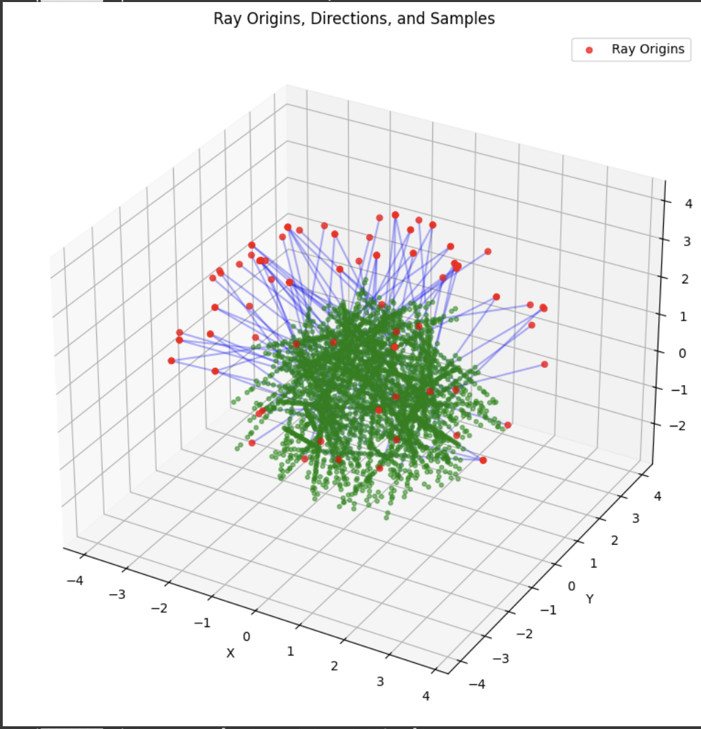
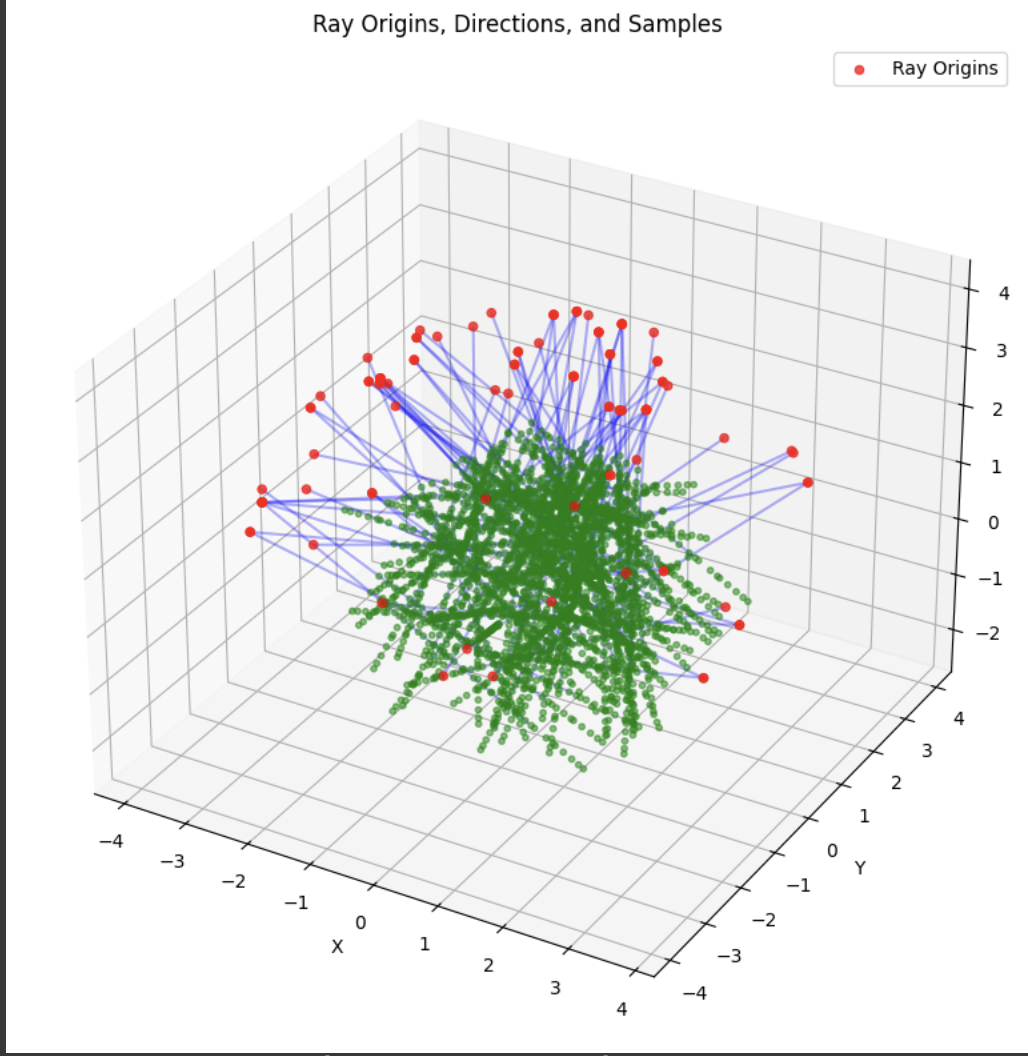
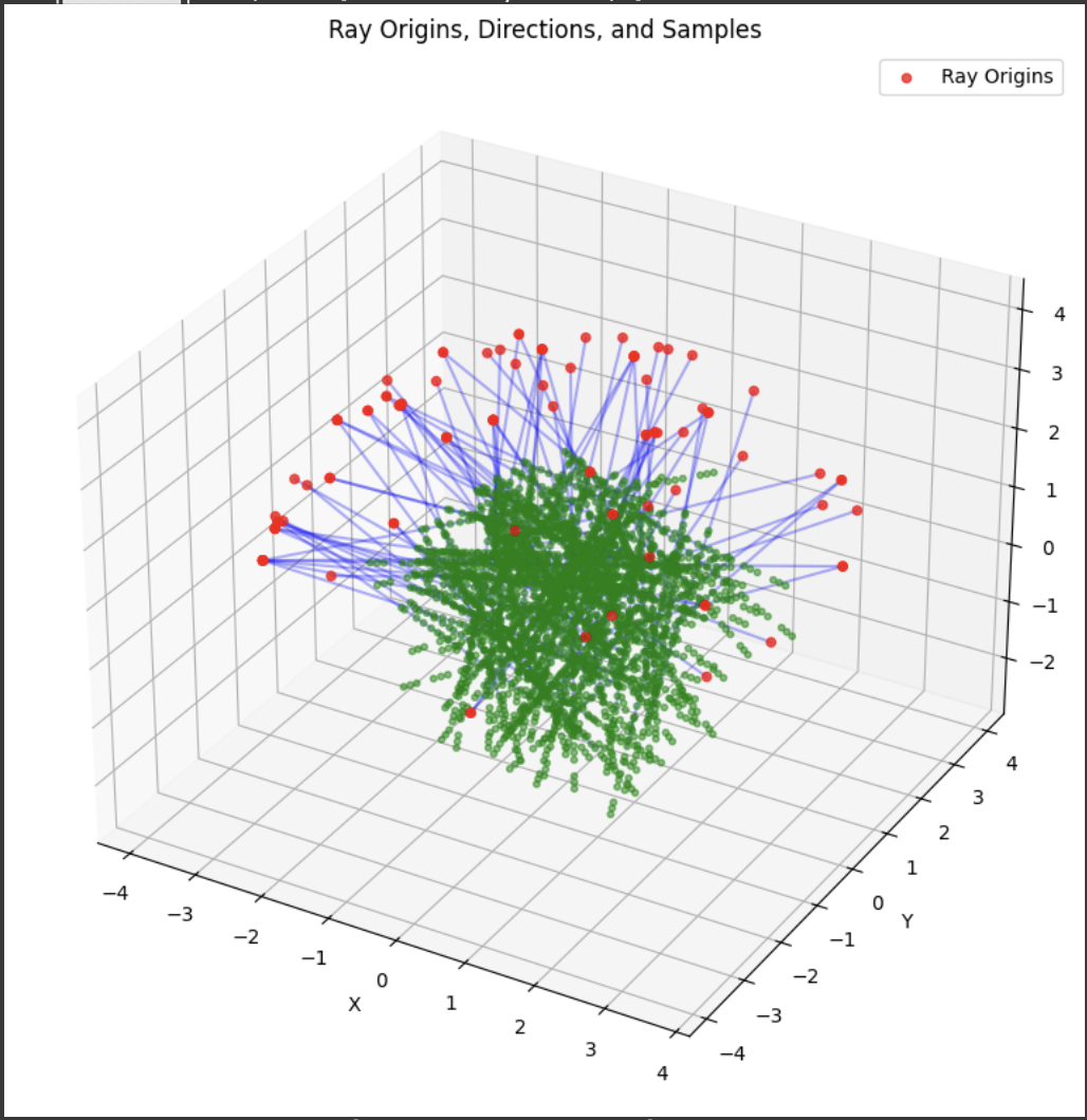
A deliverable was to show the rays and points along the rays that were sampled during training. During training, I had 10k iterations, so I just showed the results for every 1000 iterations. In my notebook code, I sampled every 100.

Part 2.4

I used the same network architecture as described in the project spec, and I got good results for it albeit the training took a while. I tried experimenting with different architectures such as CNNs to see if training would speed up, but I had way too many bugs and not enough time to do that specific B&W.

Part 2.5

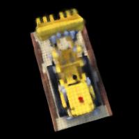
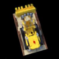
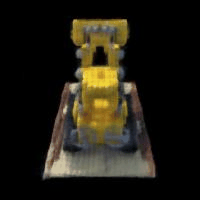
For, the volume rendering function, I just used the discrete approximation in the project spec, and I put the assert statements to test my implementation of it. I also implemented a render function to generate a novel view of the scene from a given camera viewpoint. It uses the trained NeRF model to predict color and densities, and renders the images using the volume rendering equation. This was used for visualization during the training process and after training as well. For the training, I used 10k iterations and in each iteration sampled 10k rays. For validation, I sampled 1000 rays. Here are the results of these visualizations during the process.

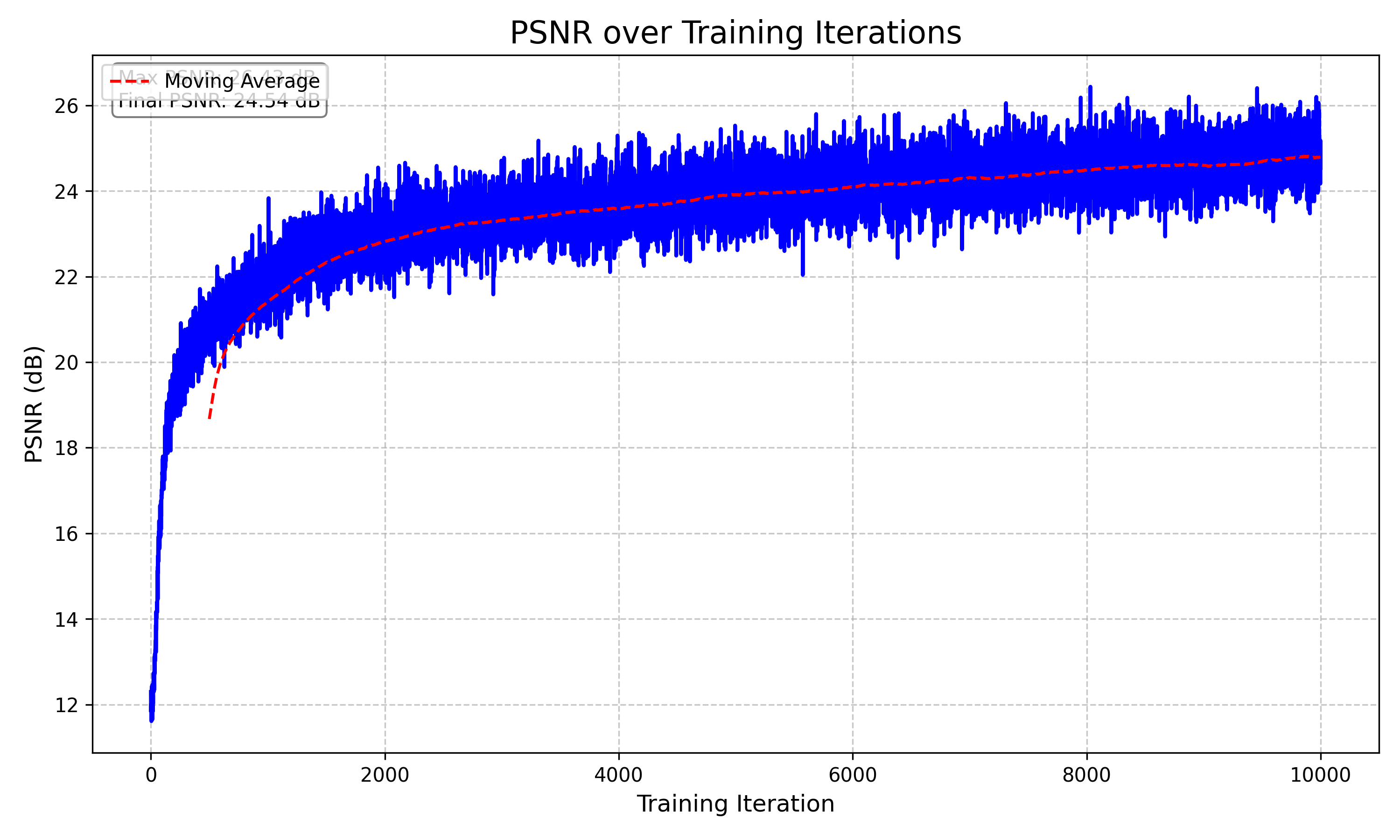
Here is the validation PSNR curve over the training iterations. I couldn't figure out my legends kept on stacking over each other, but you can clearly see that we achieve average 23 dB around 4000 iterations. I used the same learning rate as the staff solution (5e-4).

I create a GIF function that basically found all the test rendered images and sorted through them to find the correct order and created a GIF. Here is the final output. This took about an hour and half to train. I think you achieve way better results if you set the number of iterations to 20k, but I don't have that compute or credits for google colab. Also google colab times out after 5 hours when I tried on 20k iterations.

B&W

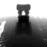
Since this project was done on my own, I implemented one bells and whistles (and the NeRF project counted for 2). I chose to do the depth map, which was covered in lecture a little bit when talking about multi-camera setups. A depth map is a visual representation that captures the distance of each pixel from the camera in a scene, effectively creating a grayscale image where darker regions represent closer objects and lighter regions represent more distant objects. The depth map is produced by generating a grid of rays from the camera through each pixel and sampling multiple points along these rays. The NeRF model, which has been pre-trained on the scene, predicts density values for each sample point, allowing the algorithm to calculate weighted depths. By passing the 3D sample points and their corresponding ray directions through the neural network, the code computes a sophisticated depth estimation that considers the density and opacity of points in the scene. The final depth map is then normalized to ensure the values range between 0 and 1, creating a visually interpretable representation of spatial depth.

The following is the result of the GiF produced of the depth maps.