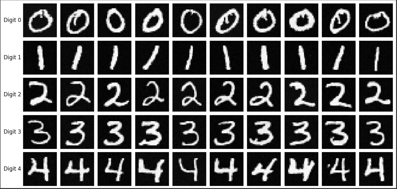
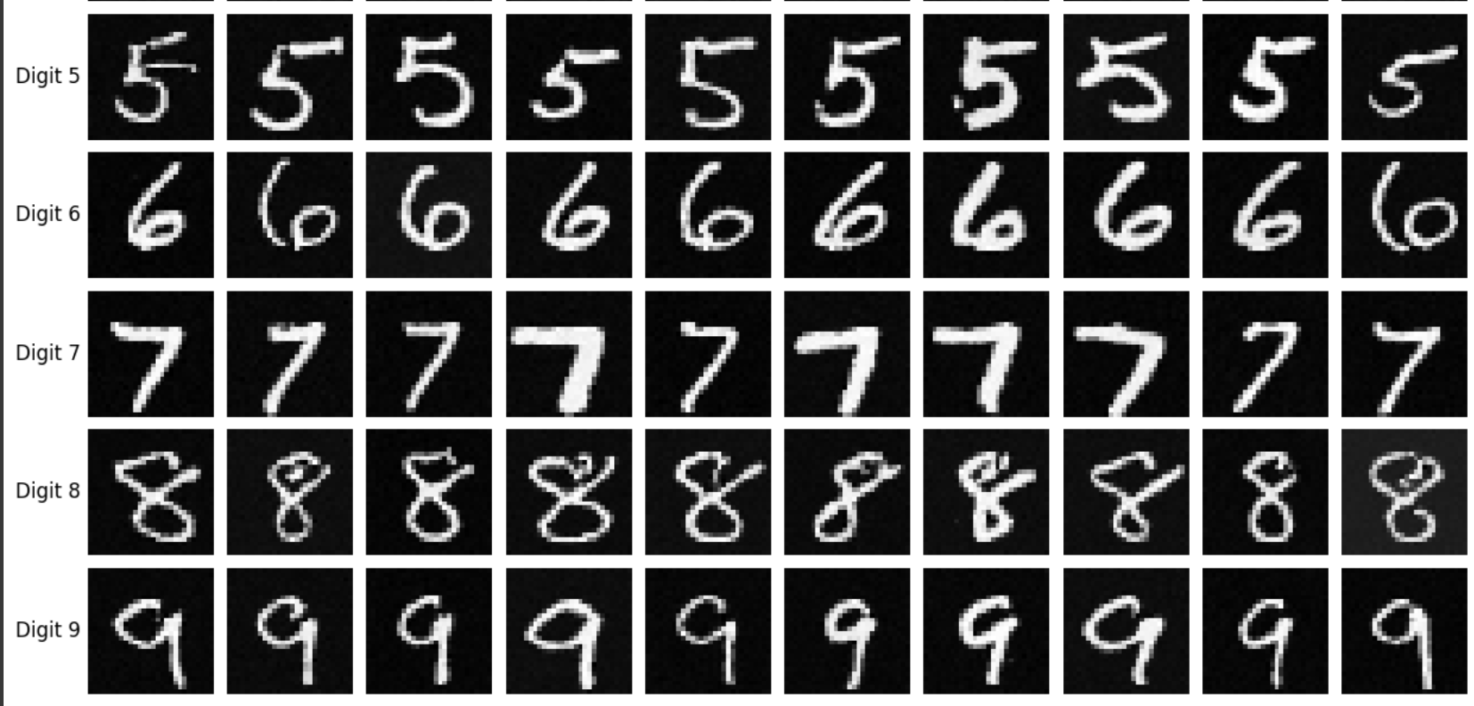
CS180 Project 5a: The Power of Diffusion Models
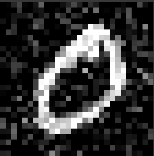
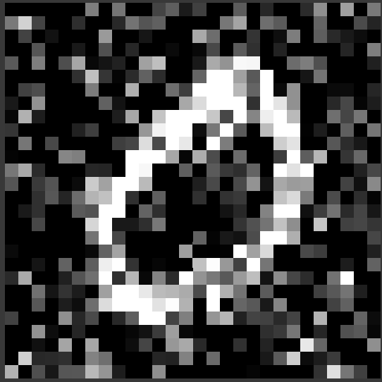
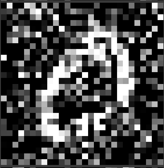
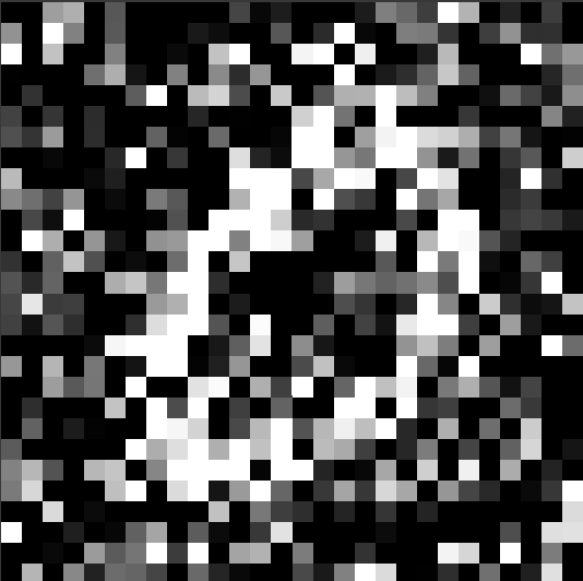
Part 1: Implementing the Forward Process
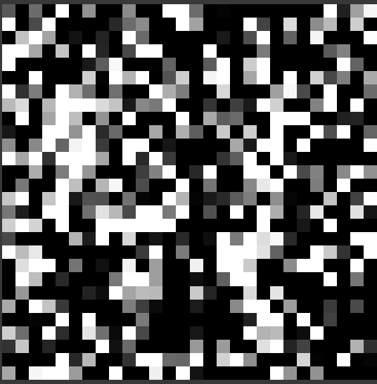
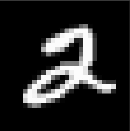
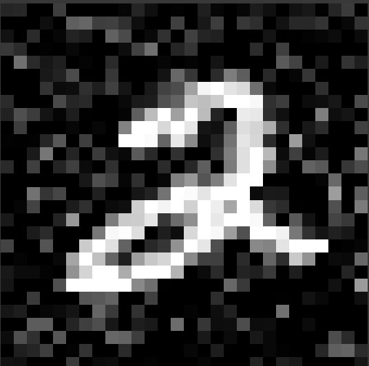
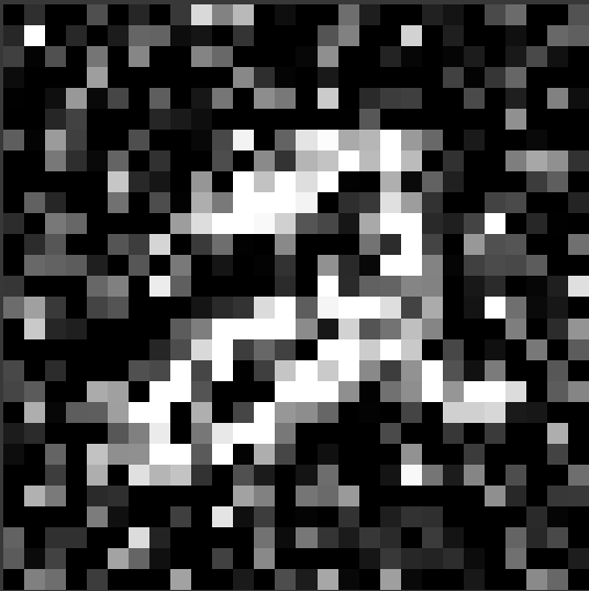
The forward process takes a clean image and adds noise to it. This is equivalent to the following:
$$x_t = \sqrt{\bar{\alpha}_t} x_0 + \sqrt{1 - \bar{\alpha}_t} \, \epsilon$$
where \( \epsilon \sim N(0, 1) \). The first square root term scales the clean image and it decreases over time as t increases, meaning the resultant image is more noisy for larger t. The second term adds gaussian noise to the image. Epsilon needs to be the same size as the original image, and each pixel is independently sampled from a normal distribution.
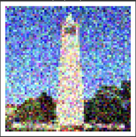


Part 2: Classical Denoising
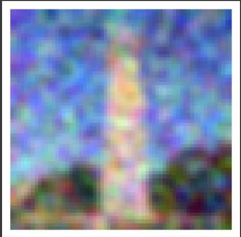
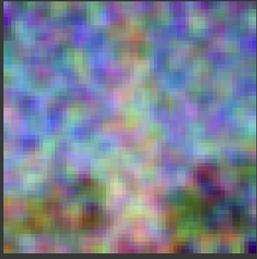
Gaussian Blurring removes high-frequeuncy compents (which noise usually is) by smoothing out the image with neighboring pixels getting larger weight. I used a sigma value of 1.5 with kernel size of 5. The results are below, but we see this isn't effective because gaussian blur is just a weighted average at a high level. This means when your image is more noisy, doing weighted averages will still have a lot of noise since there's less and less of the original image.

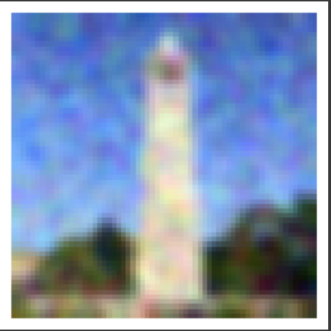


Part 3: Implementing One Step Denoising
We can rearrange the equation in part 1 to estimate the original image (assuming we know what the noise is).
$$x_0 = \frac{1}{\sqrt{\bar{\alpha}_t}} x_t - \frac{\sqrt{1 - \bar{\alpha}_t}}{\sqrt{\bar{\alpha}_t}} \, \epsilon$$
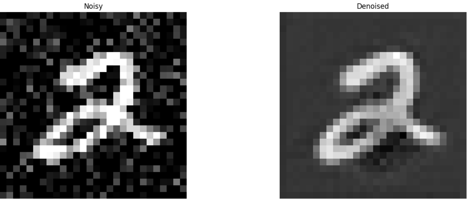
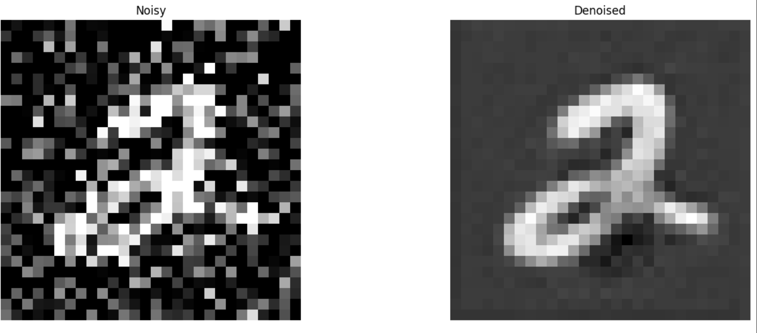
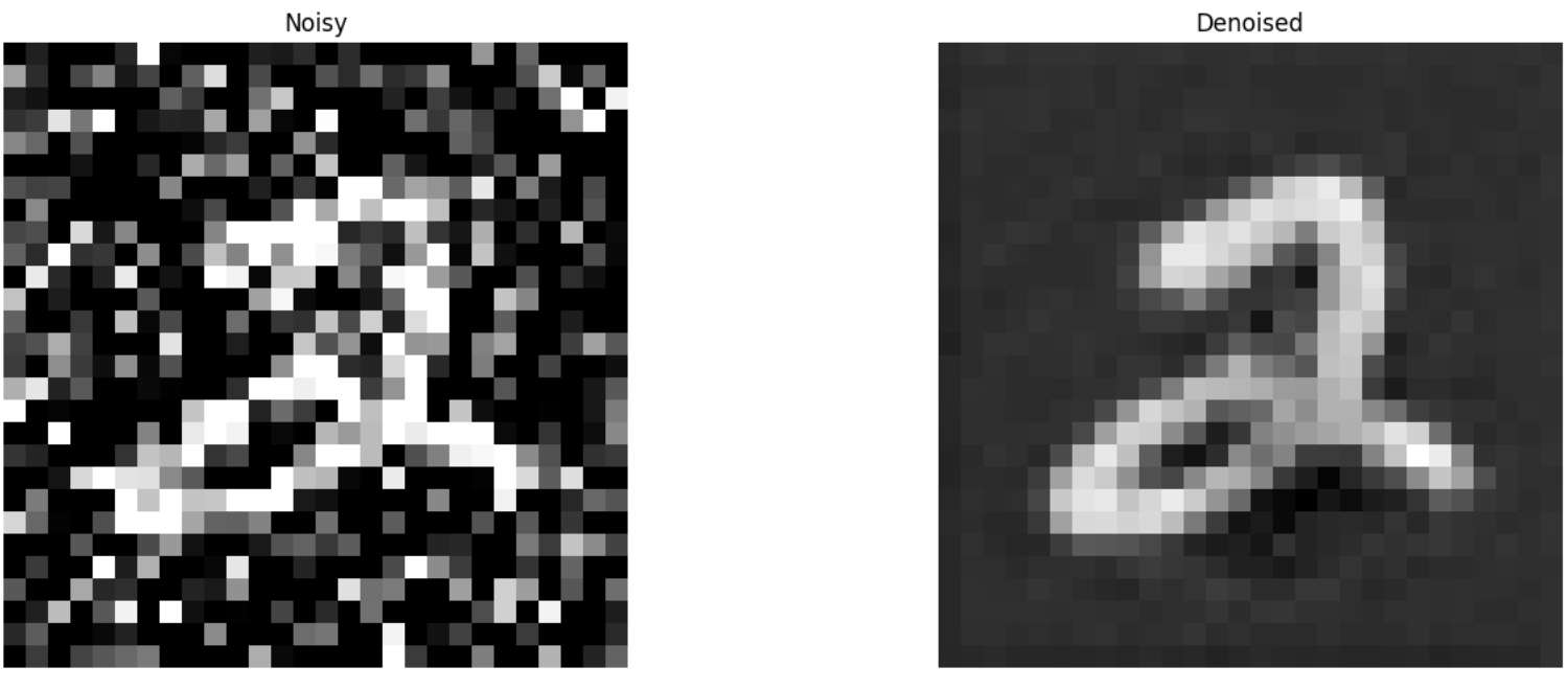
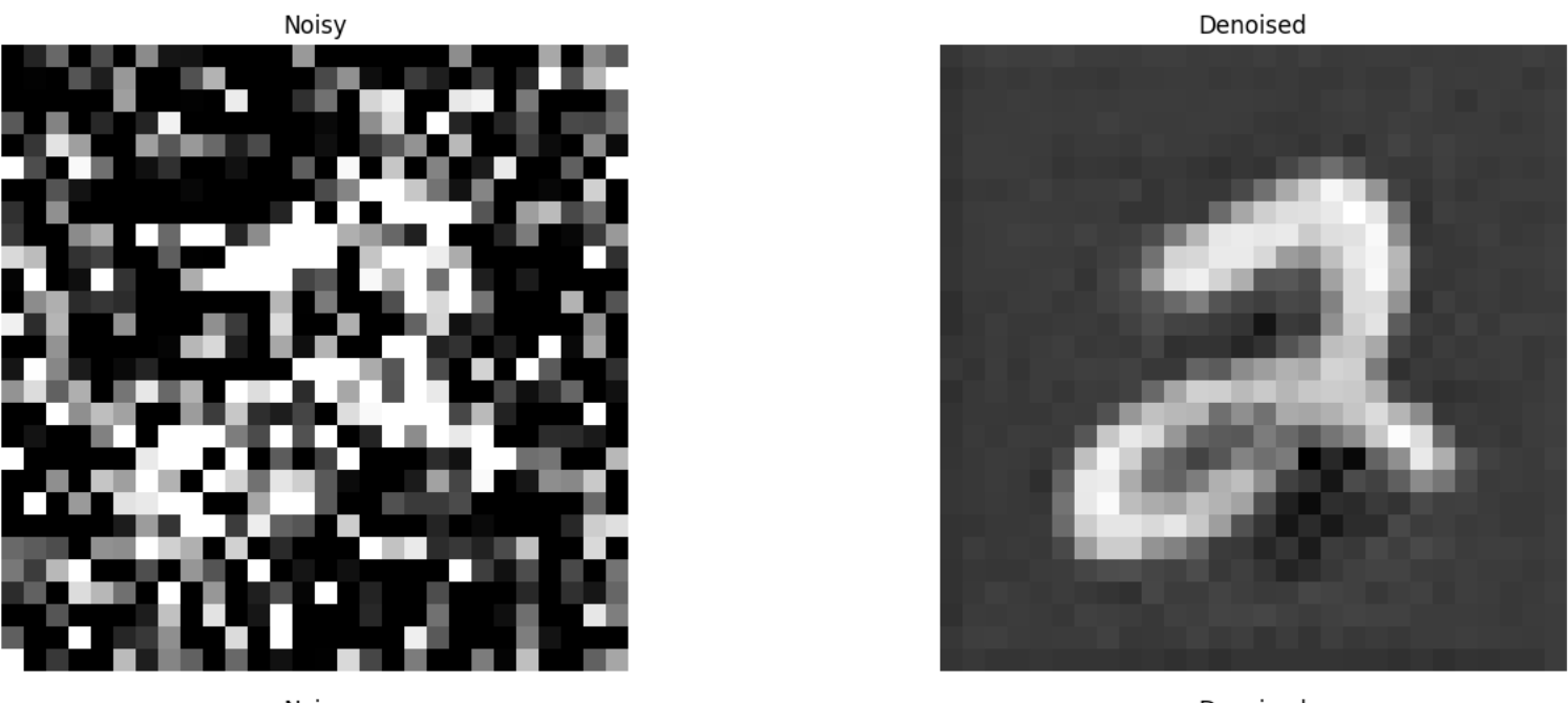
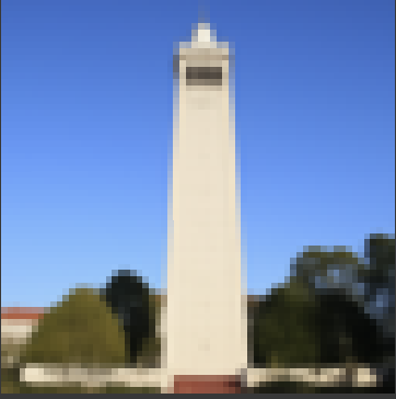
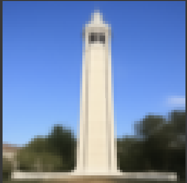
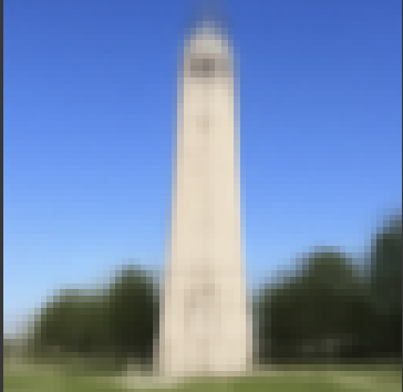
We can use a pre-trained diffusion model to get the noise estimate, and using the image above we can obtain an estimate to the original image. The results are shown below.



Part 4: Iterative Denoising
From the previous part, we see that the diffusion model predicting the noise and us solving for the original image does a much better job of projecting the noisy image on the natural image manifold. However, it clearly does worse as we add more noise. We can solve this problem iteratively by breaking it down into smaller problems. This means we start from the original noisy image then we make the result progressively less noisy. We can do this in steps of 30 to be less expensive relative to using a step size of 1.
\[x_{t'} = \frac{\sqrt{\alpha_t\beta_t}}{1-\bar{\alpha}_t}x_0 + \frac{\sqrt{\alpha_t(1-\bar{\alpha}_{t'})}}{1-\bar{\alpha}_t}x_t + v_\sigma\]
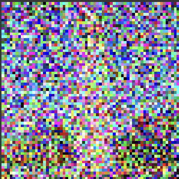
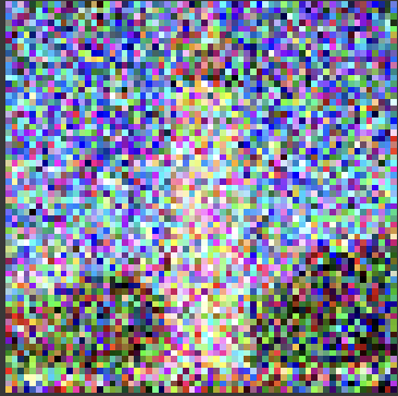
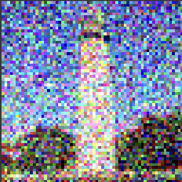
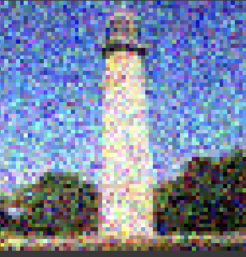
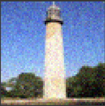
Here's the results in each 5th iteration of the denoising loop with the ones being earlier in the denoising loop.
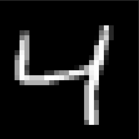
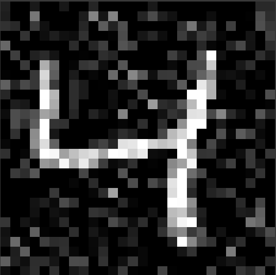
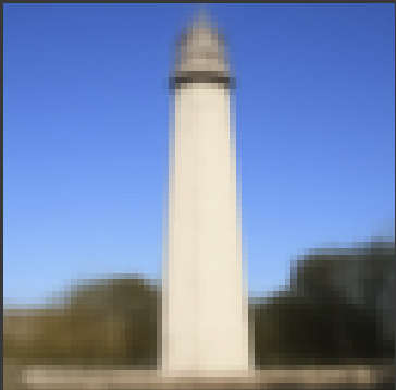
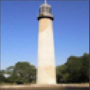
Here are the results for the one-step denoising, gaussian denoising, and final result for the iterative denoising
Part 5: Diffusion Model Sampling
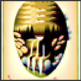
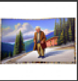
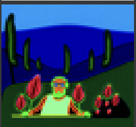
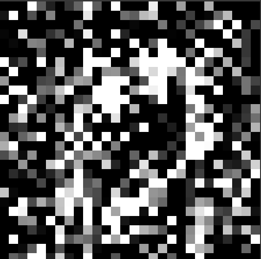
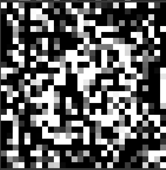
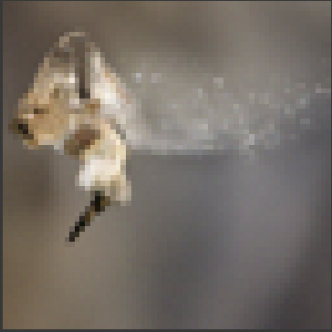
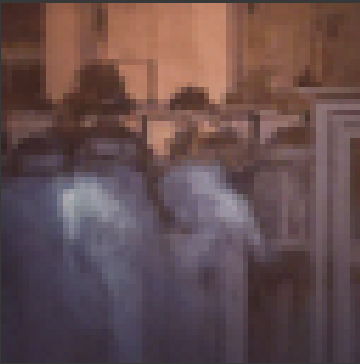
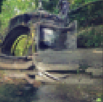
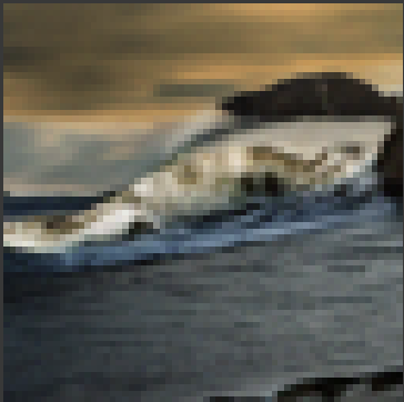
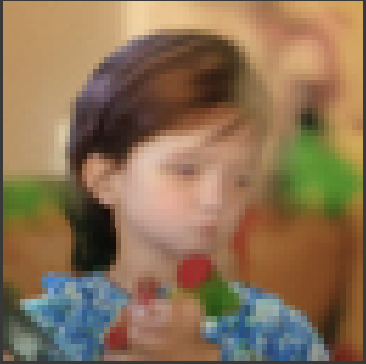
If we start from i_start = 0 and pass in random noise, we can denoise pure noise using the iterative_denoise function made from before. Here are the results. As we can see it's hard to tell what some images even are (like the 2nd and 3rd). Despite this being a 64x64 image (so the resolution is not that great), we should still be able to tell what the image is.
Part 6: Classifier-Free Guidance (CFG)
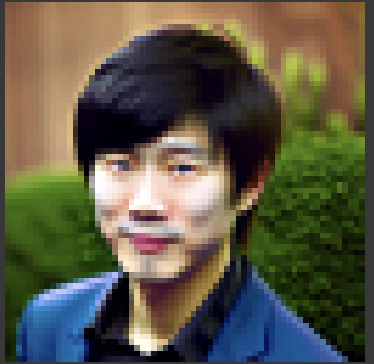
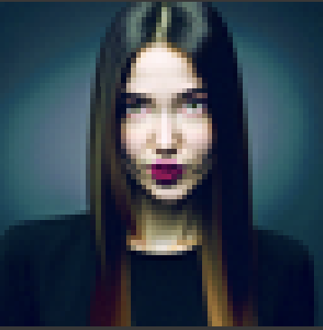
\[\epsilon = \epsilon_u + \gamma(\epsilon_c - \epsilon_u)\]
When estimating the noise, a higher lambda will result in a noise more closely following the conditional noise (meaning the resultant image is closer to the conditional text prompt). This helps the diffusion model generate images that are of higher quality (following the text prompt). The results are below.
Part 7: Image-to-image Translation
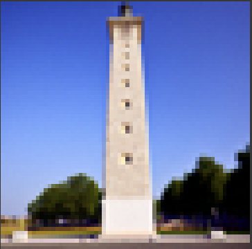
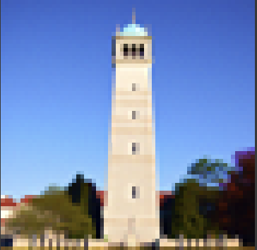
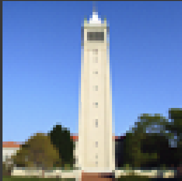
When we add more noise to the original image, we force the model to hallucinate new things so the denoising process will result in different image (since new things were hallucinated). We can see the results of the different i_start values with higher i_start meaning less noise. I also added an i_start of 30 for good measure.
Part 7.1: Editing Hand-Drawn and Web Images
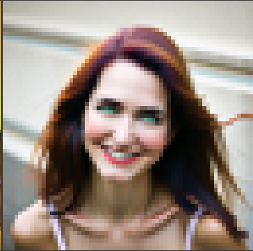
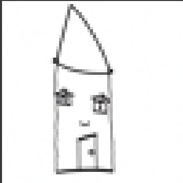
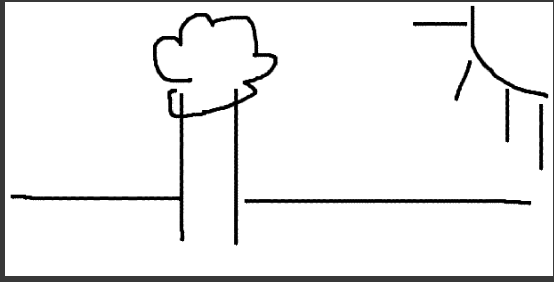
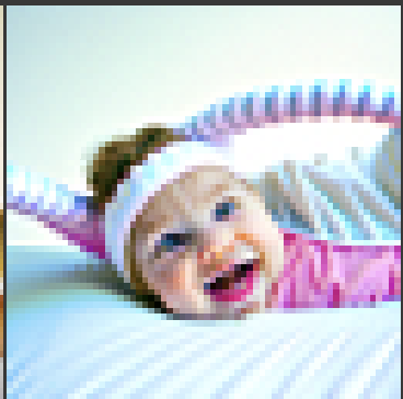
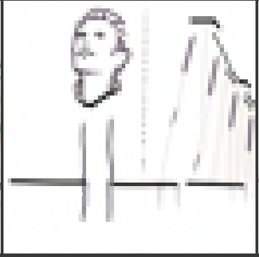
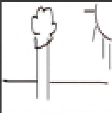
We run the same code as the last part just on 1 image from the web and 2 scribbles. All three images are non-realistic and should have better results.
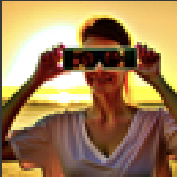
Here is our results for our first scribble of a house

Here is our results for our second scribble of a tree and a sun.

Part 7.2: Impainting
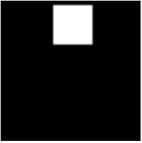
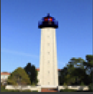
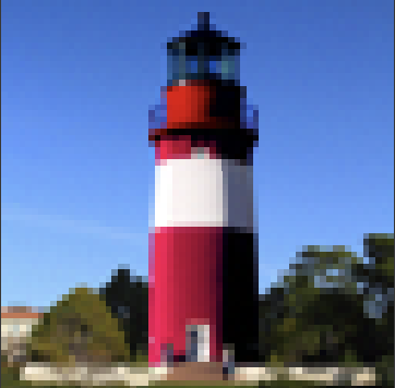
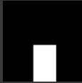
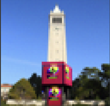
Using the formula above in each iteration of denoising, we can force certain pixels to be the same as xorigin through masking. Here are some masks and results.

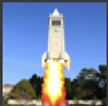
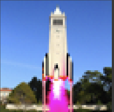
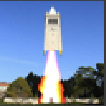
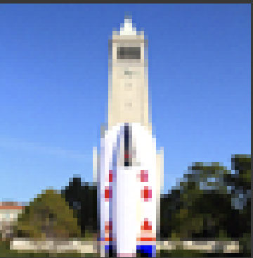
Part 7.3: Text-Conditional Image-to-Image Translation
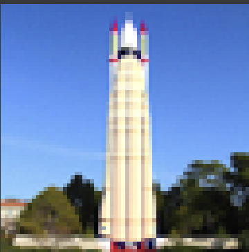
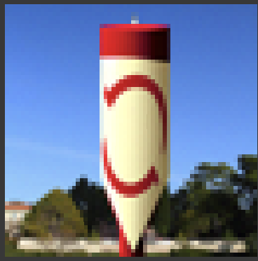
We now change the prompt to guide the resultant image projection with text.
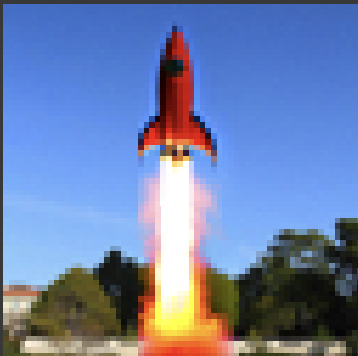
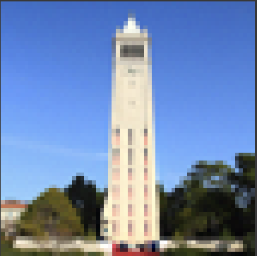
For our first text prompt: "a rocket ship" with a rectangular mask covering the whole campanile.
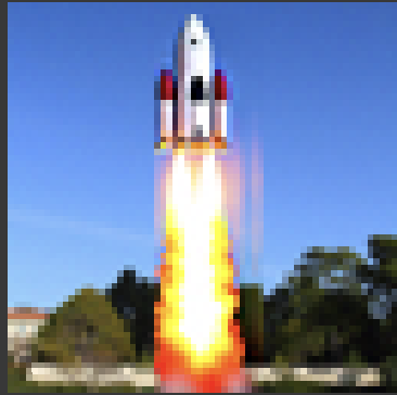
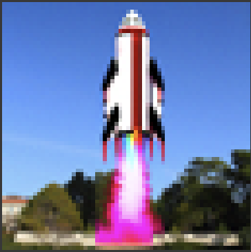
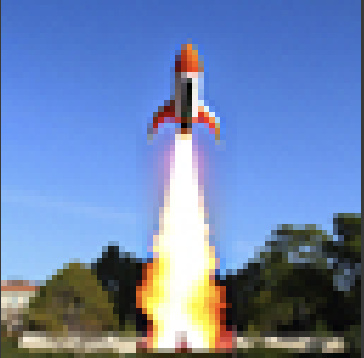
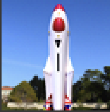
For our second text prompt: "a pencil" with a rectangular mask covering the whole campanile.
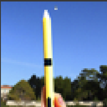
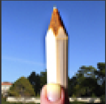
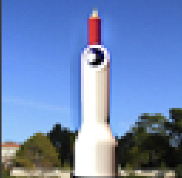
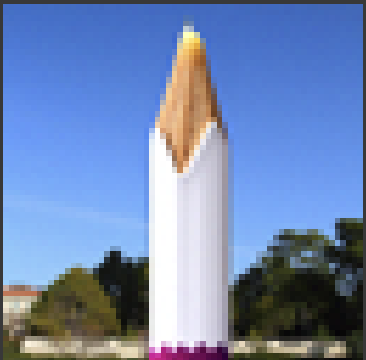
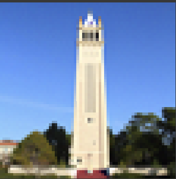
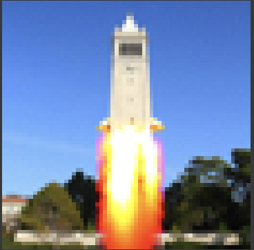
For our third text prompt: "a rocket ship" but this time just a mask on the bottom half of the campnanile.
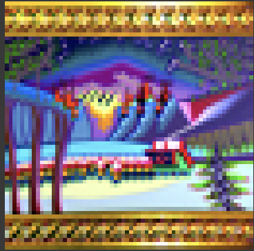
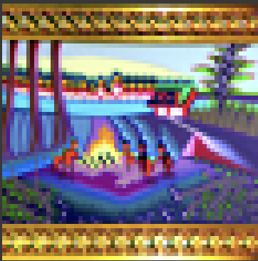
Part 8: Visual Anagrams
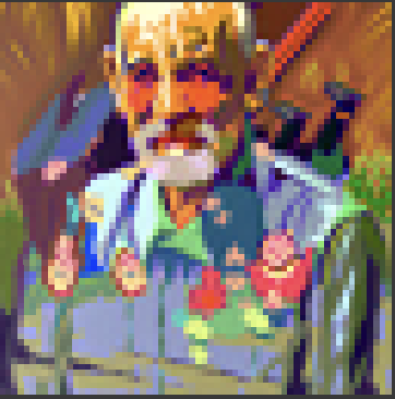
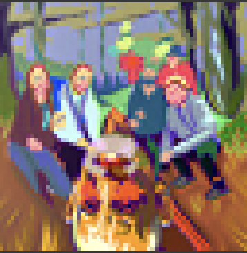
Our goal is to create a single image that looks like one thing in its normal orientation and another thing when flipped. This requires two prompts (one for each orientation). The key idea is we are trying to force each orientation to like each prompt. We already know how to do this normally through iterative denoising. Inside each iterative denoising loop, we need to also calculate the noise in the flipped direction. We need to average the two noises along with the variances. A key part is to flip the noise of the other orientations. This is because we add the noise back in the normal orientation.

Part 9: Hybrid Images
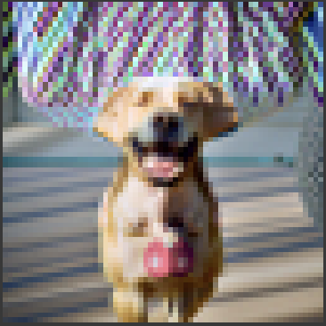
In order to create hybrid images, we need to get to do a lowpass filter and get the low frequency noise estimate of one image and the high frequency noise estimate of another image. We combine these values to get a new hybrid noise estimate. We can implement the low frequency and high frequency noise estimates using the gaussian filter. Here are some results.
