Part 1: Recovering Homographies

Homographies are used as transformation matricies to map points from one plane to another. We need to use homogenous coordinates to allow for more complex projections. You can use least-squares to solve for the homography, but I used SVD as it is a better way to avoid the case where H is near singular (making the SVD solution more robust than least-squares). The math is also shown below.

The matrix-vector multiplication is:

$$ \begin{pmatrix} x' \\ y' \\ w' \end{pmatrix} = \begin{pmatrix} h_{11} & h_{12} & h_{13} \\ h_{21} & h_{22} & h_{23} \\ h_{31} & h_{32} & h_{33} \end{pmatrix} \begin{pmatrix} x \\ y \\ 1 \end{pmatrix} = \begin{pmatrix} h_{11}x + h_{12}y + h_{13} \\ h_{21}x + h_{22}y + h_{23} \\ h_{31}x + h_{32}y + h_{33} \end{pmatrix} $$

The resulting equations are:

$$ x' = h_{11}x + h_{12}y + h_{13} $$ $$ y' = h_{21}x + h_{22}y + h_{23} $$ $$ w' = h_{31}x + h_{32}y + h_{33} $$

To convert back to Cartesian coordinates \( (x_c, y_c) \), divide by \( w' \):

$$ x_c = \frac{x'}{w'} = \frac{h_{11}x + h_{12}y + h_{13}}{h_{31}x + h_{32}y + h_{33}} $$ $$ y_c = \frac{y'}{w'} = \frac{h_{21}x + h_{22}y + h_{23}}{h_{31}x + h_{32}y + h_{33}} $$

Part 2: Warping

For warping, I found the homography using the source and destination points defined by the correspondences, and I used that to warp the source points to the destination points. I used inverse warping and nearest-neighbor interpolation.

Part 3: Rectification

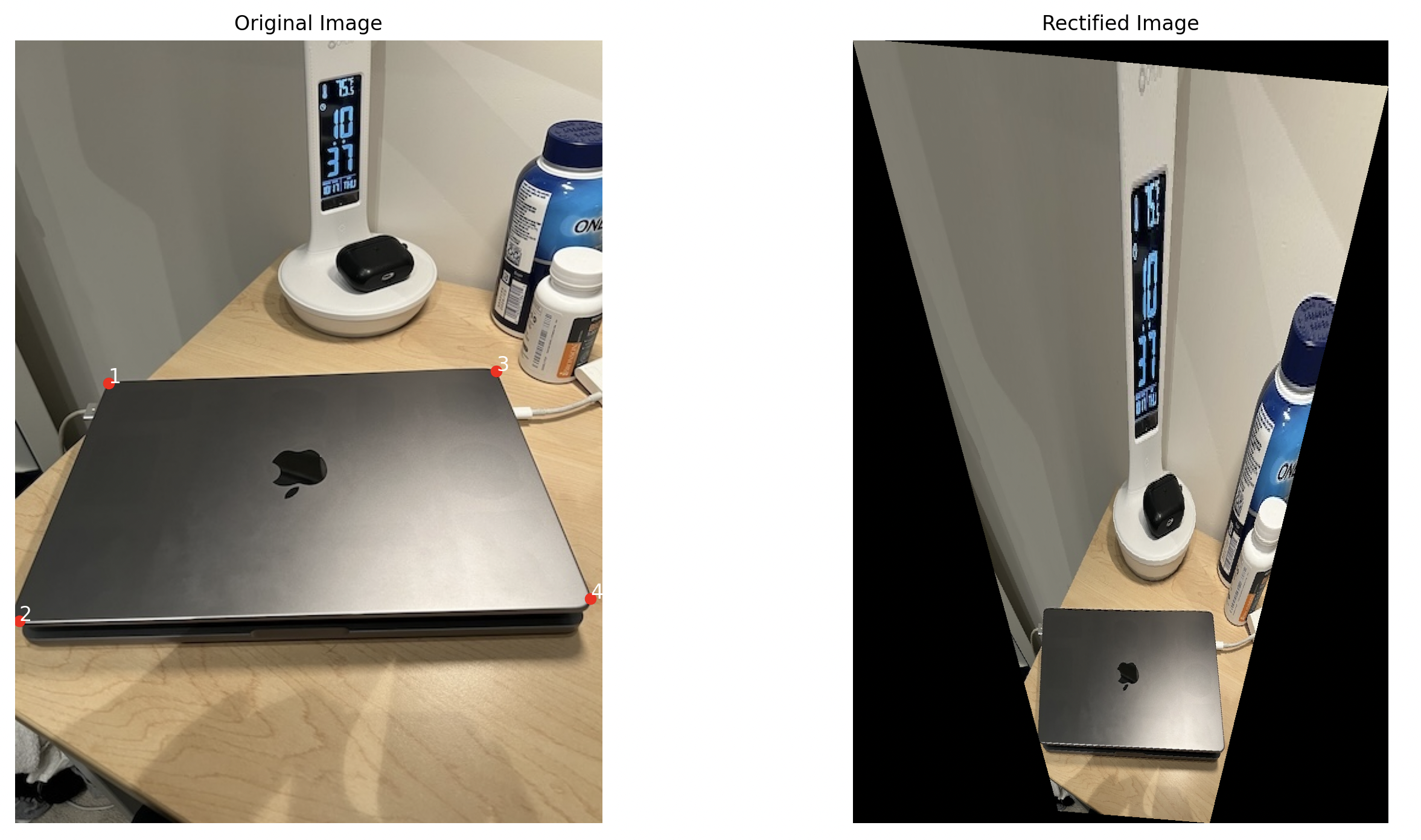
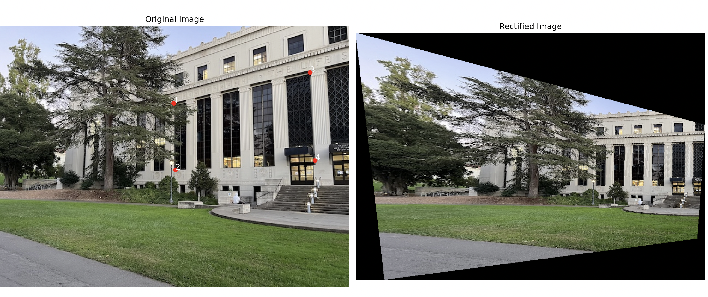
This part involves perspective changing the shape of a rectangular object in the input (which may be at an angle), and shifting it so that it appears like a flat rectangle in the output. I utilized the correspondence tool from last time. Results are show below.

Part 4: Blending The Images Into a Mosaic

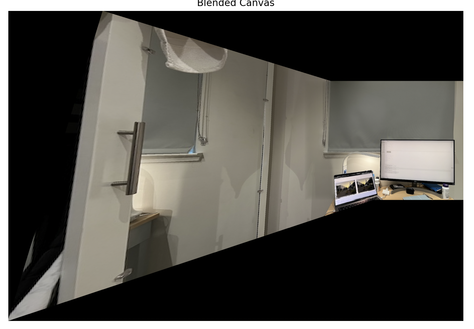
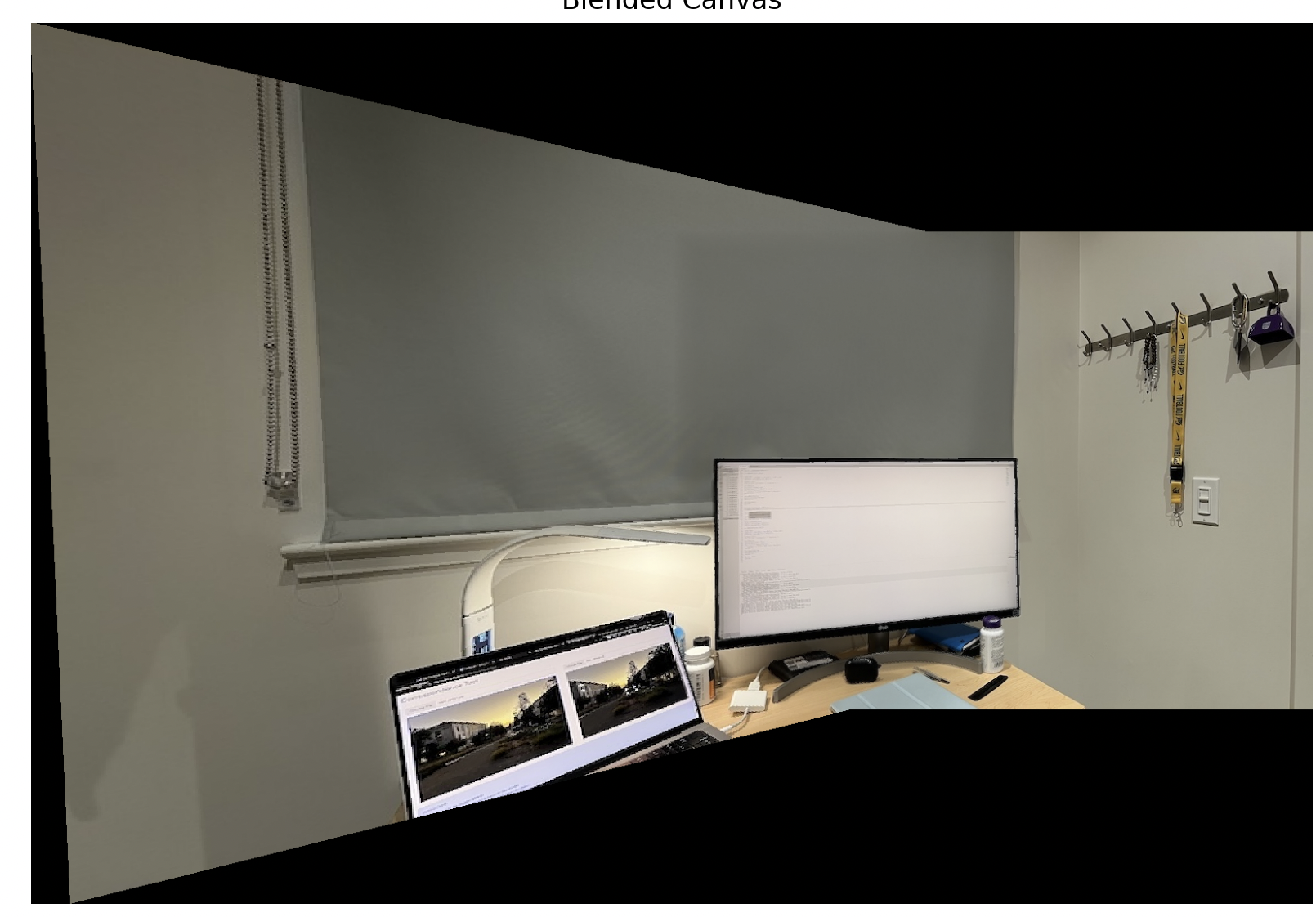
In this two-image mosaic process, there are two main steps: image warping and alignment, followed by blending the images to remove visible seams. To ensure that the combined images fit within the same frame, I created a larger canvas that is big enough to hold both warped_im1 and im2. This canvas accounts for any translation or displacement that occurs during the warping process, ensuring both images are positioned properly within the same coordinate space.

I created binary masks for both warped_im1 and im2. A binary mask is simply a black-and-white image where the white areas represent the visible portions of the image, and the black areas represent the background or unused space. To create these masks, I converted the images to grayscale and then applied a thresholding technique. Pixels above a certain threshold are set to 255 (white), while others are set to 0 (black). This process allows me to distinguish between the foreground (image content) and the background. I computed distance transforms for each mask. A distance transform calculates, for each pixel, how far it is from the nearest boundary (edge of the image content). The result is a smooth gradient of values where pixels near the edges of the image content have a value close to 0 (since they are right at the boundary) and pixels further away from the edges, towards the center of the image content, have values closer to 1.

The next step was to calculate an alpha mask. If dist_mask2 is larger, the pixel will primarily be taken from im2. In areas where the images overlap, the alpha mask ensures a gradual blend by weighting the two images according to their relative distances from the edges. I preserved the non-overlapping areas by directly copying the content from warped_im1 and im2 into the final canvas

$$ \alpha = \frac{{\text{{dist_mask1}}}}{{\text{{dist_mask1}} + \text{{dist_mask2}} + \epsilon}} $$

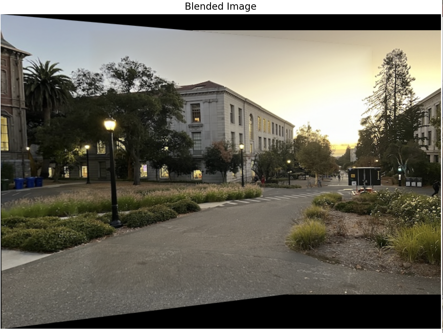
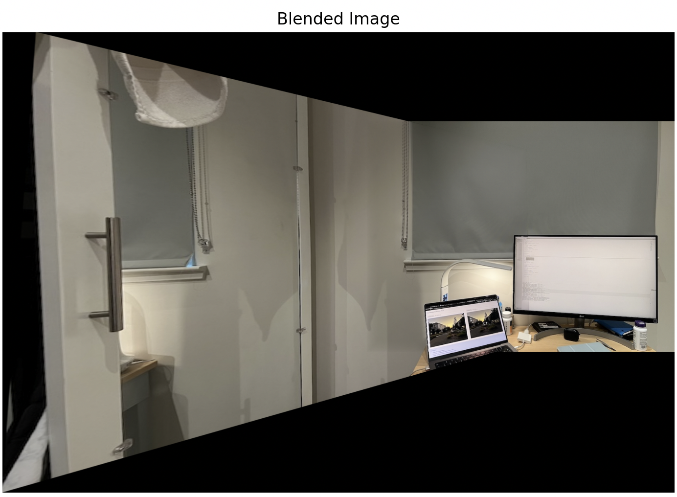
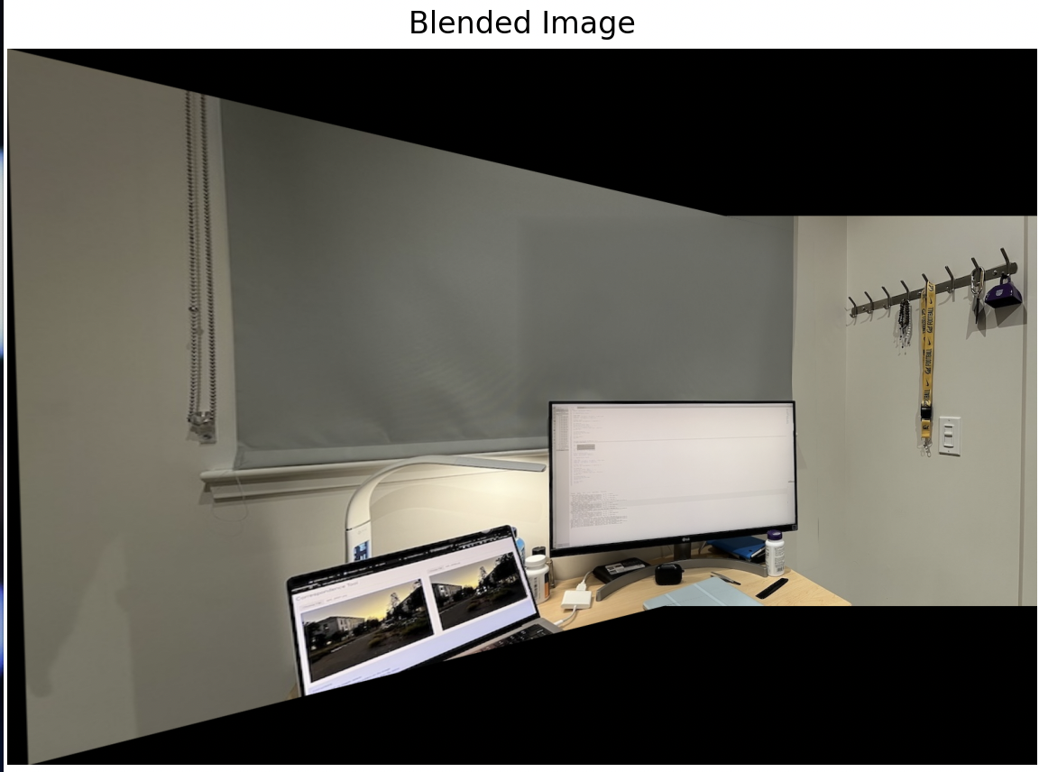
These are the close ups of the panoramics.

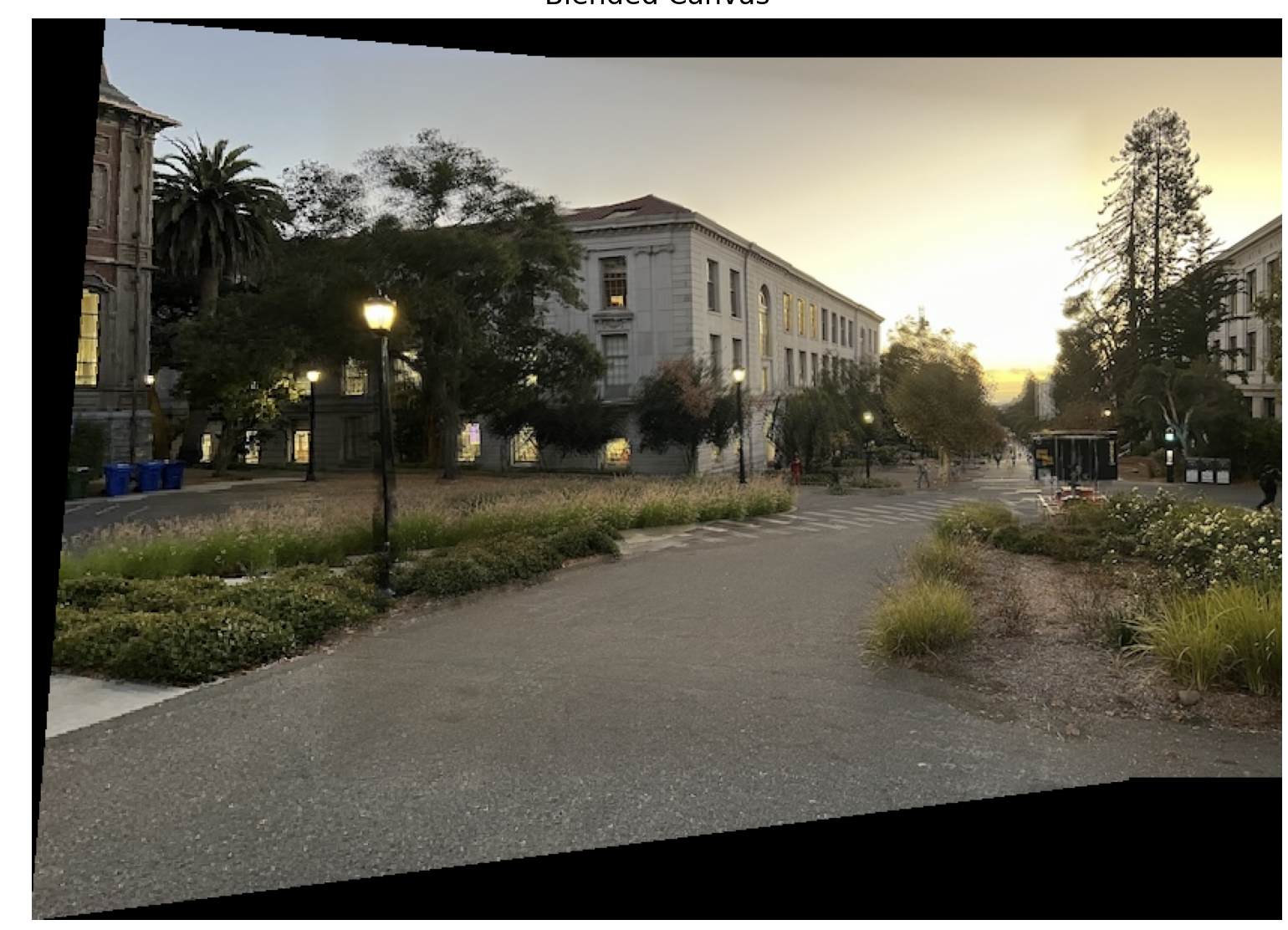
These are the side by side of the source images + panoramics.

Part 1: Harris Corners

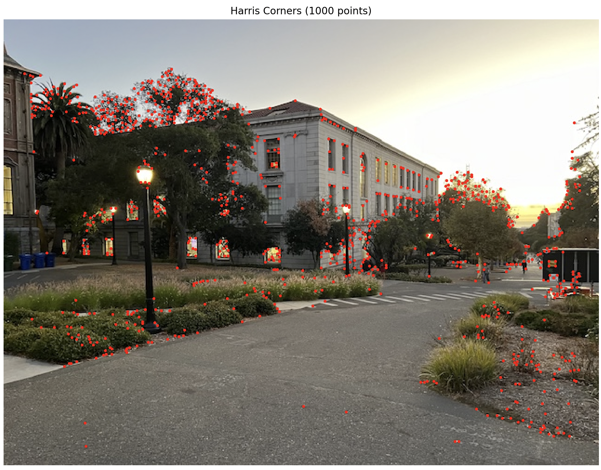
The Harris Corner Detection algorithm starts by computing the image gradients in the horizontal and vertical directions. These gradients capture how pixel intensities change in the x and y directions.

Next, a second moment matrix (also known as the structure tensor) is built over a small window around each pixel. This matrix summarizes the changes in intensity based on the gradients and describes how much variation occurs in different directions.

• Corners: If the pixel is at a corner, both eigenvalues of the matrix will be large, as the intensity changes significantly in multiple directions.
• Edges: For an edge, the intensity changes significantly in one direction but not the other, so one eigenvalue will be large, while the other will be close to 0.
• Flat Regions: In flat areas, both eigenvalues will be small, as there is little to no variation in intensity.

The Harris Response score \( R \) is calculated using the eigenvalues of the second moment matrix. A common formulation is:

\[ R = \frac{\text{det}(M)}{\text{trace}(M)} = \frac{\lambda_1 \lambda_2}{\lambda_1 + \lambda_2} \]

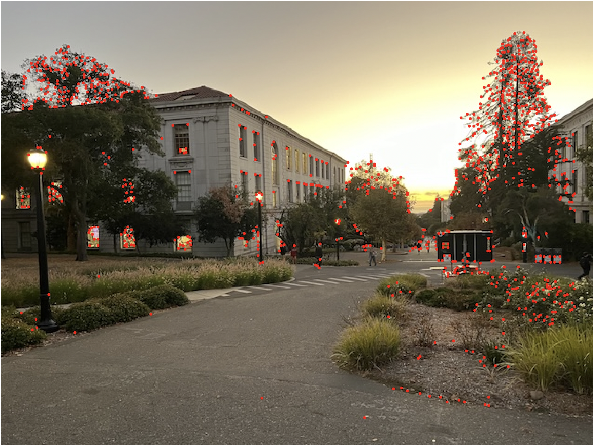
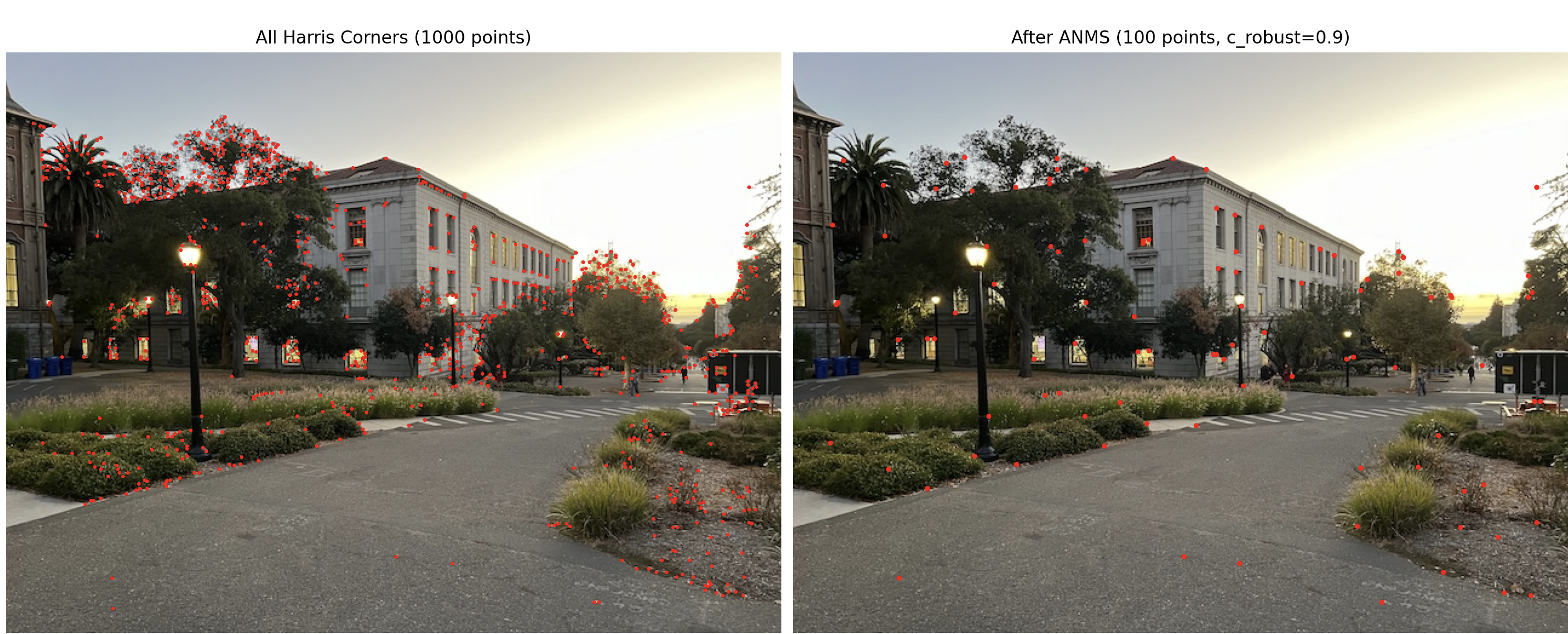
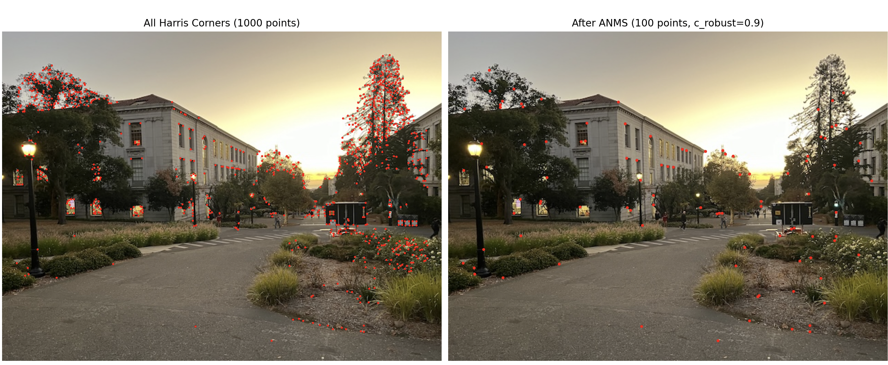
This score does a good job of distinguishing corners (where both eigenvalues are large) from edges (where one eigenvalue is large and the other is small) and flat regions (where both eigenvalues are small). I used the code provided in the project description with the addition of filtering through the response values to choose the best 1000 points.

Part 2: Adaptive Non-Maximal Suppression

$$r_i = \min_j |\mathbf{x}_i - \mathbf{x}_j|, \text{ s.t. } f(\mathbf{x}_i) < c_{\text{robust}}f(\mathbf{x}_j), \mathbf{x}_j \in \mathcal{I}$$

Adaptive Non-Maximal Suppression (ANMS) selects a subset of points while using a criterion that determines which points are considered "locally" better. A stronger point in the paper presented is considered a point j (relative to point i) is such that the following equation holds true: f(j) > c_robust * f(i)

I looped through each point and found all the ecludian distances between the current point i and all the other points. I then created a boolean array indetifying, which tells us what points are stronger than point i. I found the minimum distance to the nearest stronger point, and used that value to determine the strongest 100 points. A higher minimum distance means that this is a very locally strong point relative to its neighbors, while a low minimum distance menas that this point is locally very weak relative to its neighbors. Using this, we find sort by the minimum distances, selecting the points associated with the largest minimum distances.

Part 3: Feature Descriptor

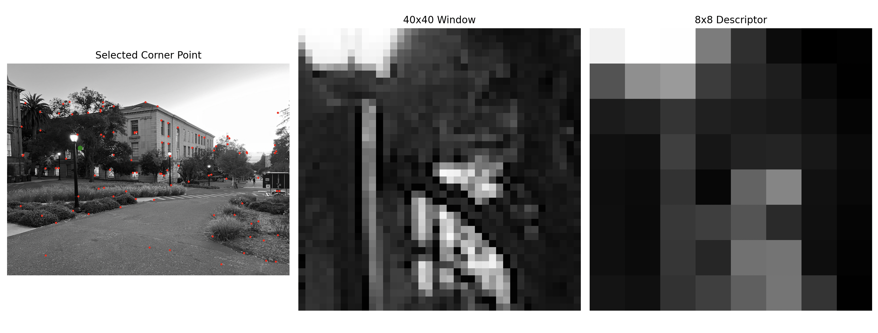
A feature descriptor is a concise representation of the local information around a feature point in an image. It captures essential visual characteristics of the area surrounding the feature point that is invariant to different changes like constrast, rotation, and lighting (which is why it's useful for our specific task). To create a feature descriptor for a feature point, a small region of the image around this point (a patch) is extracted. In this case, we extract a 40x40 pixel window around the feature point. The next step is to downsample this window to an 8x8 because a smaller patch will reduce sensitivity to noise and small variations while still capturing the overall pattern in the region of interest. The way we do this is (after doing a gaussian blur of the 40x40 region) we take every 5th pixel to fill the 8x8 patch. We also normalize this resized patch to remove the effects of any changes in lighting or contrast. The way we do this is through bias noramlization which is just subtracting the mean pixel value from each pixel in the patch to adjust for any brightness differences. Then we do gain normalization which is dividing by the norm of the patch to scale the pixels correctly regardless of any contrast differences. The result for one corner point selected after ANMS is shown.

Part 4: Feature Matching

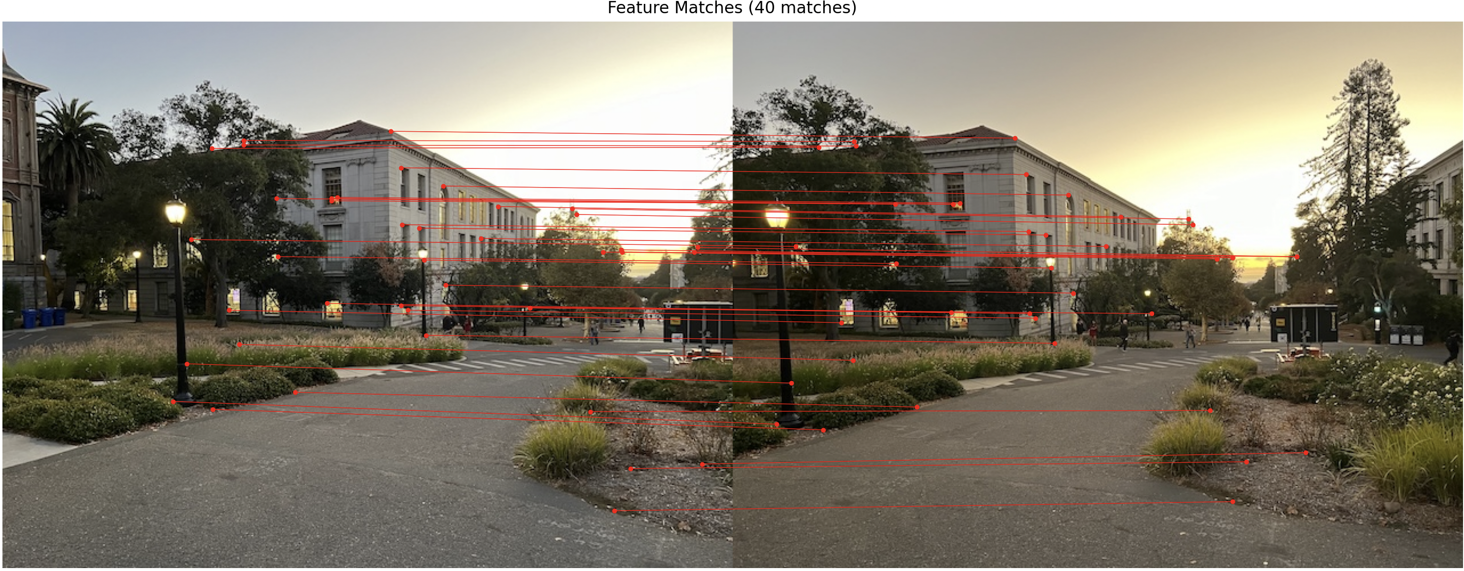
We create feature descriptors for each feature point in each image. For each descriptor in the first image, we compute the Euclidean distance between that discreptor and all descriptors in the second image. We find the closest and the second closest descriptors from the second image. A match is considered valid if the ratio of the closest distance / second closest distance is under a ratio threshold. The idea is that the closest match should be significantly closer than the second-closest match, which helps filter out poor feature matches. The result is shown below.

Part 5: RANSAC

Despite Lowe's ratio test filtering out many outliers, some incorrect feature pairs still remain. If we were to use a least-squares method, it wouldn’t be robust to these outliers—just one bad feature match could skew the homography result significantly. This is where RANSAC (Random Sample Consensus) becomes valuable. RANSAC allows us to handle outliers by iteratively sampling a small set of points. We repeatedly select four random point pairs and compute the homography using only these pairs. Then, we determine the number of inliers for the homography. After many iterations, we select the homography with the most inliers, which represents the best alignment while ignoring outliers.

For my specific implementation, I split it up into three functions. The first function is called compute_homography, and it computes the homography using SVD given a set of source and destination points. If we set the last element of the last row of H to be 1 (to ensure we have unique homography since you can scale the matrix to get infinitely many solutions), then you have 8 unknowns, meaning a minimum of 4 points is required (since each point has a corresponding equation for the x and y coordinate).

The second function is called compute_homography_error. This is used to determine if any given corresponding point is an inlier or not. It averages the forward error (dist(H*p1, p2)) and the backward error dist((H_inverse *p2, p1)) as the result.

The main pipeline of the RANSAC is in the ransac_homography function. This is where the main logic of updating the best homography (the one with the most inliers) is done and stored. The best homography is returned. This function can be turned for the error threshold and number of iterations. I used 2000 for the number of iterations with error_threshold of 5 pixels. I copied my code from part a of the project to do the same exact blending and stitching of images. The results are shown below side by side. The left side is results from part A, and the right side are the results from autostitching.

Favorite Thing

The coolest thing about the project was automating the feature matching and stitching because I ended up getting less blurry results since my manual feature matching wouldn't be exact (human error).