Face Morphing

Part 1: Defining Correspondences

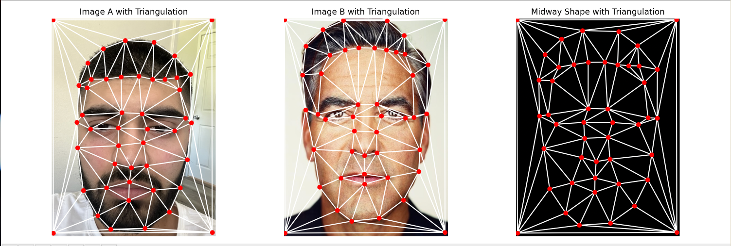
We select key corresponding features such as eyes, nose, hairline, etc., to define corresponding points to the two images. I selected around 40 points. Now, we can compute the midway shape by taking the average of these corresponding points. We can also visualize the triangle mesh created by a Delaunay triangulation algorithm for the original face, the desired face, and the midway face. Why do we use the Delaunay algorithm? Because it maximizes the angles in the triangle, which means we don't have "skinny triangles". Skinny triangles are no good as you have an uneven pixel distribution. I.e., when you are mapping pixels from the source triangle to the skinny triangle, you are going to be smearing a lot of the pixels over the same area, which loses a lot of detail. The results of the triangulation are below.

Part 2: Computing the "Mid-Way Face"

For computing affine translations of traingles, we can solve it using a system of linear equations. \[ \begin{pmatrix} x'_1 \\ y'_1 \\ x'_2 \\ y'_2 \\ x'_3 \\ y'_3 \end{pmatrix} = \begin{pmatrix} x_1 & y_1 & 1 & 0 & 0 & 0 \\ 0 & 0 & 0 & x_1 & y_1 & 1 \\ x_2 & y_2 & 1 & 0 & 0 & 0 \\ 0 & 0 & 0 & x_2 & y_2 & 1 \\ x_3 & y_3 & 1 & 0 & 0 & 0 \\ 0 & 0 & 0 & x_3 & y_3 & 1 \end{pmatrix} \cdot \begin{pmatrix} m_{00} \\ m_{01} \\ m_{02} \\ m_{10} \\ m_{11} \\ m_{12} \end{pmatrix} \]

Performing the multiplication results in the following system of equations:

\[ \begin{aligned} x'_1 &= m_{00} \cdot x_1 + m_{01} \cdot y_1 + m_{02} \\ y'_1 &= m_{10} \cdot x_1 + m_{11} \cdot y_1 + m_{12} \\ x'_2 &= m_{00} \cdot x_2 + m_{01} \cdot y_2 + m_{02} \\ y'_2 &= m_{10} \cdot x_2 + m_{11} \cdot y_2 + m_{12} \\ x'_3 &= m_{00} \cdot x_3 + m_{01} \cdot y_3 + m_{02} \\ y'_3 &= m_{10} \cdot x_3 + m_{11} \cdot y_3 + m_{12} \end{aligned} \]

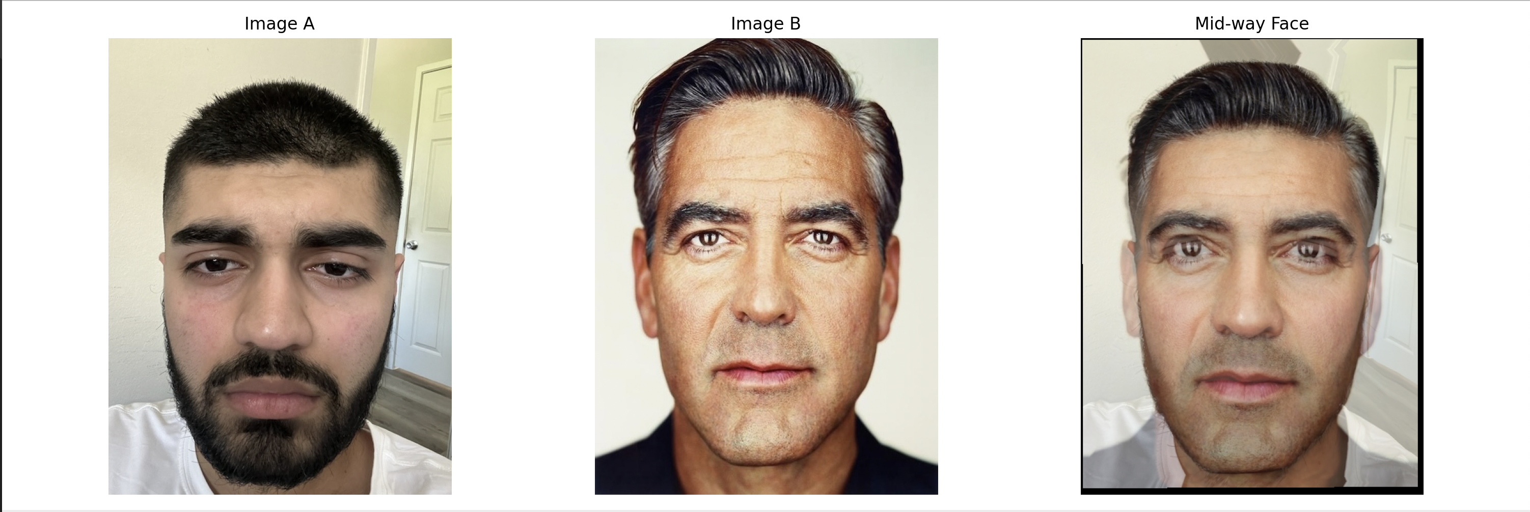
For each triangle in the mid-way face, we get the corresponding triangles from imageA and imageB. We find the affine translation from the points of the triangle from A to the midway (we do the same for B). We then warp the images using the translation. A mask is utilized to get the part we are interested in. We also accumalate these masks and normalize at the end to prevent overcontribution.

Part 3: The Morph Sequence

The bulk of the work for this problem was done in the last problem. The only thing we need to do is add the warping and dissolve fractions, to help generate a sequence of frames. These sequence of frames, once generated, can be compiled into an Mp4. I turned the Mp4 to a GIF that is displayed below.

The intermediate points are used to defined the intermediate shape that the morphed image at a certain timestep will take. A warp_frac of 0 will result in the original image shape, and increasing it will get you closer to image2 shape (with 1 being the exact shape of image2). \[ \text{points_intermediate} = (1 - \text{warp_frac}) \cdot \text{im1_pts} + \text{warp_frac} \cdot \text{im2_pts} \]

The blended warp is calculated as a weighted average. \[ \text{blended_warp} = (1 - \text{dissolve_frac}) \cdot \text{warped_im1} + \text{dissolve_frac} \cdot \text{warped_im2} \]

Part 4: The Mean Face Of The Population

I utilized the Danes dataset. I also have code that parsed the folder to split the documents based on extension type. I also parsed the ASF files for relevant information. Using that information, we calculated the average correspondences (including the corners). This provided us with the average face shape. Then we had to go through each image and morph it to the average face. I utilized the morph function from before with warp_frac = 1 since we wanted the average face structure, and I set dissolve_frac to 0. I also parsed through the JPG files to use the images that were always facing forwards (filtered on 1m).

I redid the correspondeces between my face and the average face to get the points. Warping required utilizing the morph function and setting the warp fraction parameter to either 0 or 1 based on if we wanted to morph the average shape to me or me to the average shape. We can see it works as the average face forehead resembles my forehead, and my forehead expands to morph into the average face forehead.

Part 5: Extrapolating From The Mean

\( \text{caricature_landmarks} = (1 - \alpha) \cdot \text{mean_landmarks} + \alpha \cdot \text{landmarks} \)

For any alpha > 1 we begin extrpolation. I chose two values of 1.25 and 1.5, and the results of it are shown below. We can see my nose get bigger and forehead smaller (since my features are more exaggerated).

Part 6: Bells and Whistles