Filters and Frequencies

Part 1.1: Finite Difference Operator

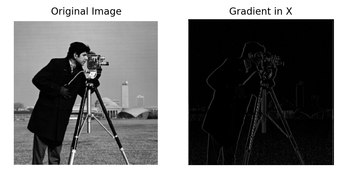
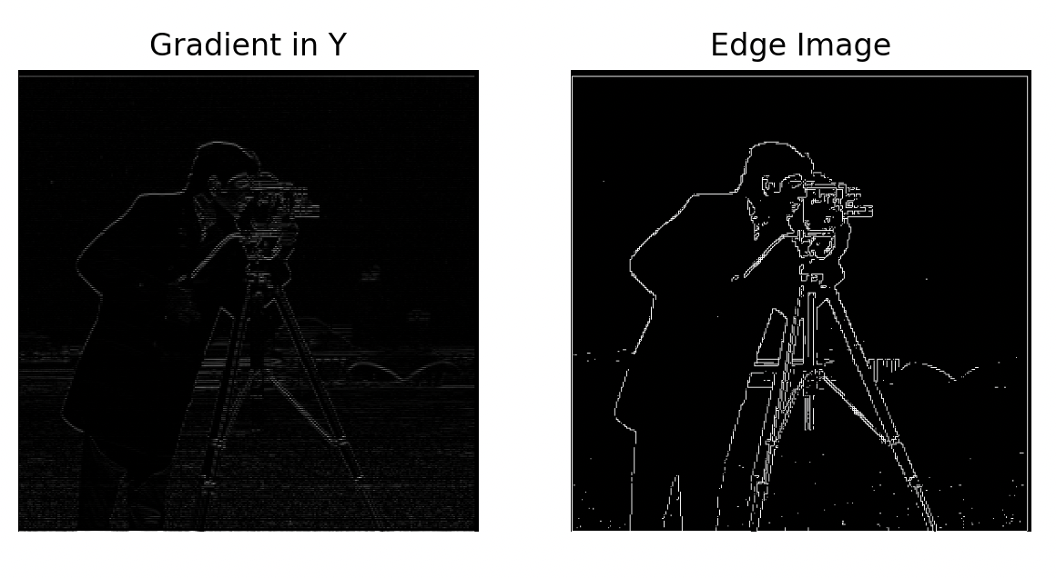
The gradient across the X dimension is convoluted with the 2D matrix [[1, -1]], which is this operation for each pixel: \( \text{Gradient}_{x}(i,j) = I(i,j+1) - I(i,j) \). The gradient across the Y dimension is convoluted with the 2D matrix [[1], [-1]], which is this operation for each pixel: \( \text{Gradient}_{y}(i,j) = I(i+1,j) - I(i,j) \). For our gradient magnitude calculation (before applying threshold), we do sqrt(Dx^2 + Dy^2). The gradient magnitude at edges is a lot greater since there's more changing in pixels at those points. We then experimentally choose a threshold to show the edges as some of the gradient magnitude is just noise. We also don't really care about the direction of the change, so we just take the abs for the grad_x, and grad_y images. Doing a 2D Convolution with the image for each of the gradients gets us the following results:

Part 1.2: Derivative of Gaussian Filter

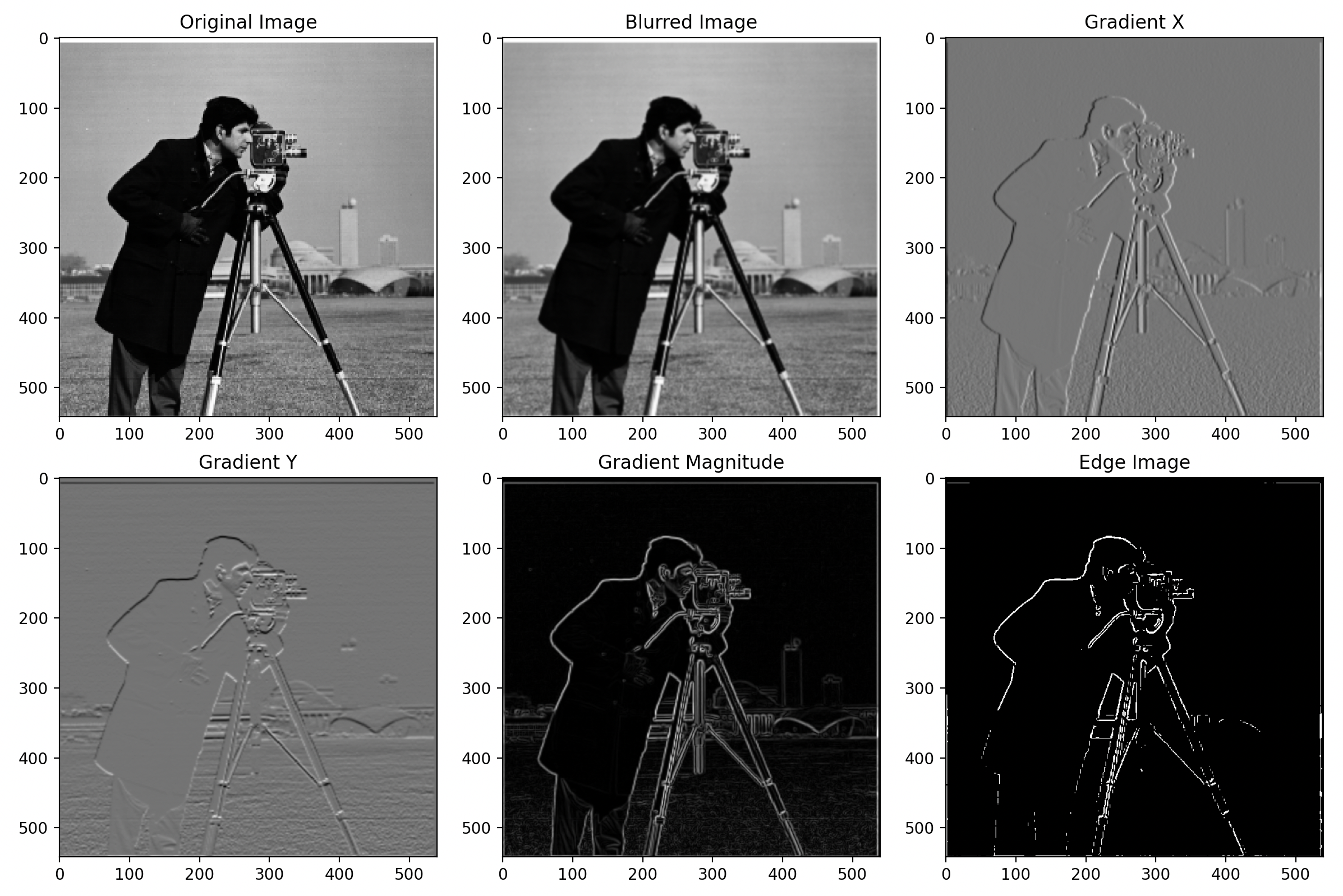
To get a 2D Gaussian, we specify a kernel size of 5 with a standard deviation 1. We then do an outer product, to get a 5x5 Gaussian Filter. This Gaussian Filter is used for convolution with the image, then we take the derivative of that output using the technique mentioned in 1.1. The difference we see is that the noise is not as visible because the random dots in the bottom quarter of picture are no longer visible.

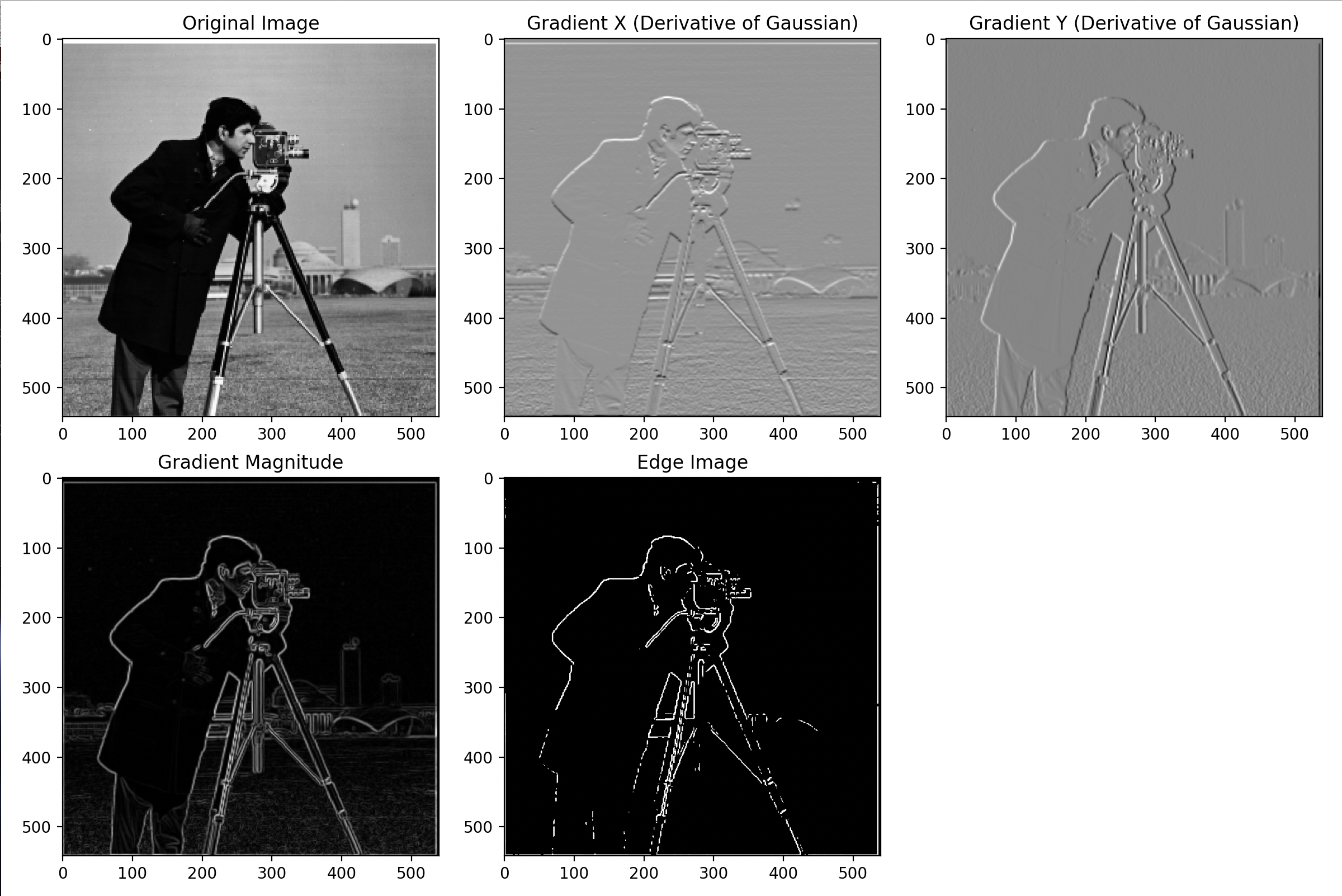
For DoG, we use a 1D derivative of a guassian with a kernel size of 5. We do the outer product, to get a 5x5 first derivative gaussian filter. We then convolve the image with the DoG. This is essentially gets us the same image as before. This works because of the mathematical properties of the convolution operator.

Part 2.1: Image Sharpening

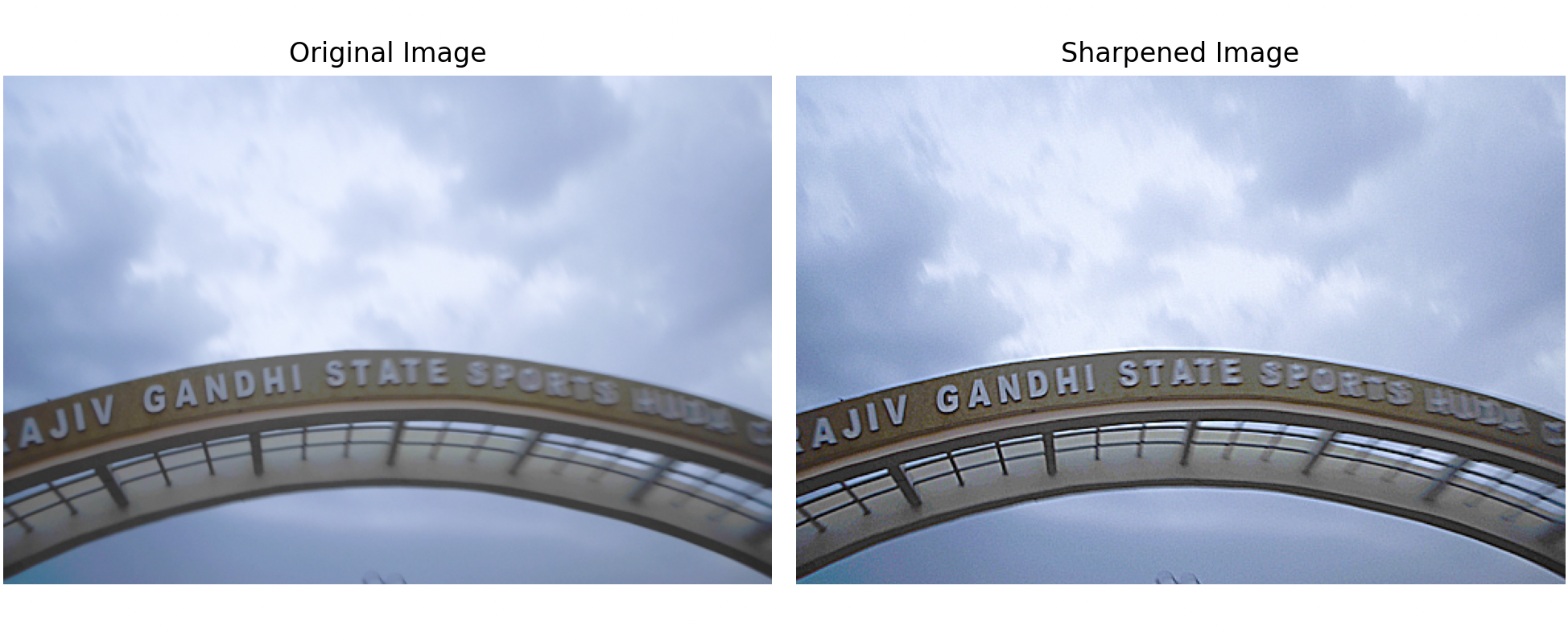
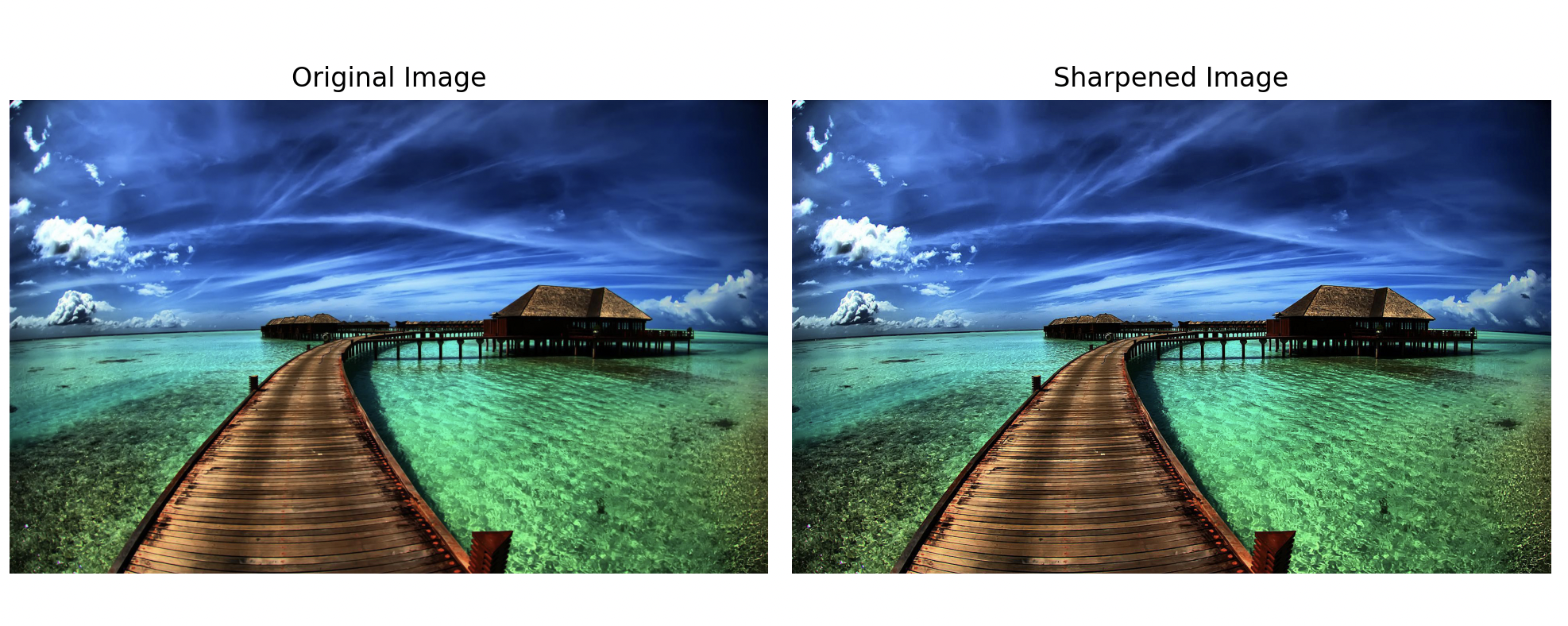
We know the Gaussian Filter smoothes the image by acting as a low pass filter. Therefore, image - gaussian filter(image) will get us the high frequencies. Adding the high frequencies (multiplied by some constant) + the original image will get us the sharpened image. We read the pixels in as a float to ensure arithmetic precision, but need to clip it into uint8 (0-255) range to plot the image. The third image is the high res image sharpened. As expected, we can't really see much difference. The default constant factor is 1.5 used in all of the image sharpening.

Part 2.2: Hybrid Images

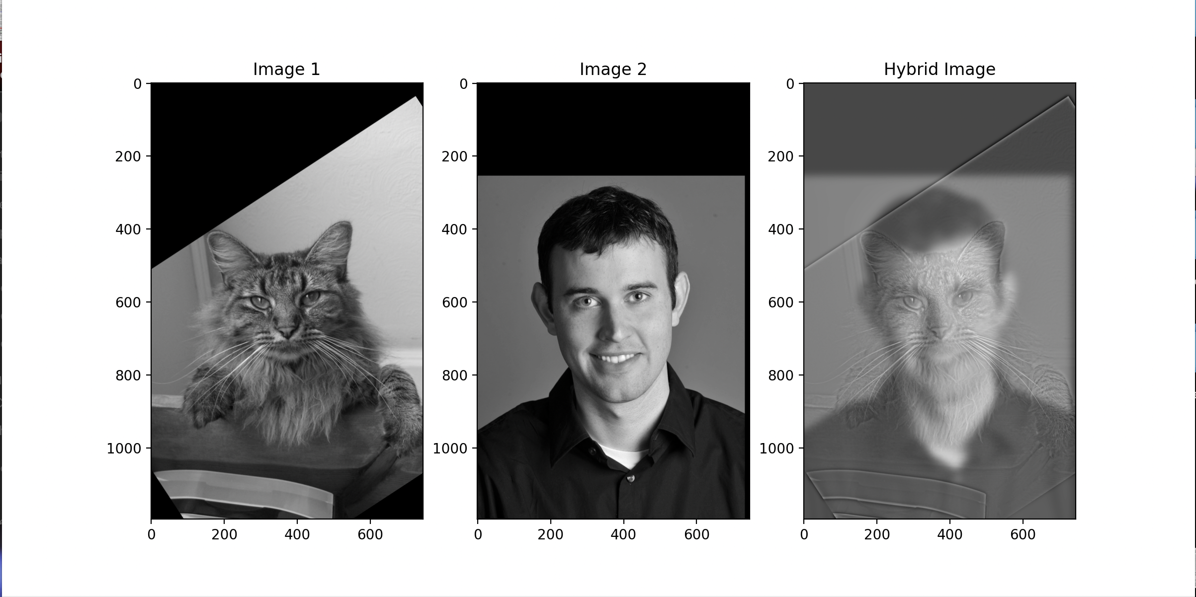
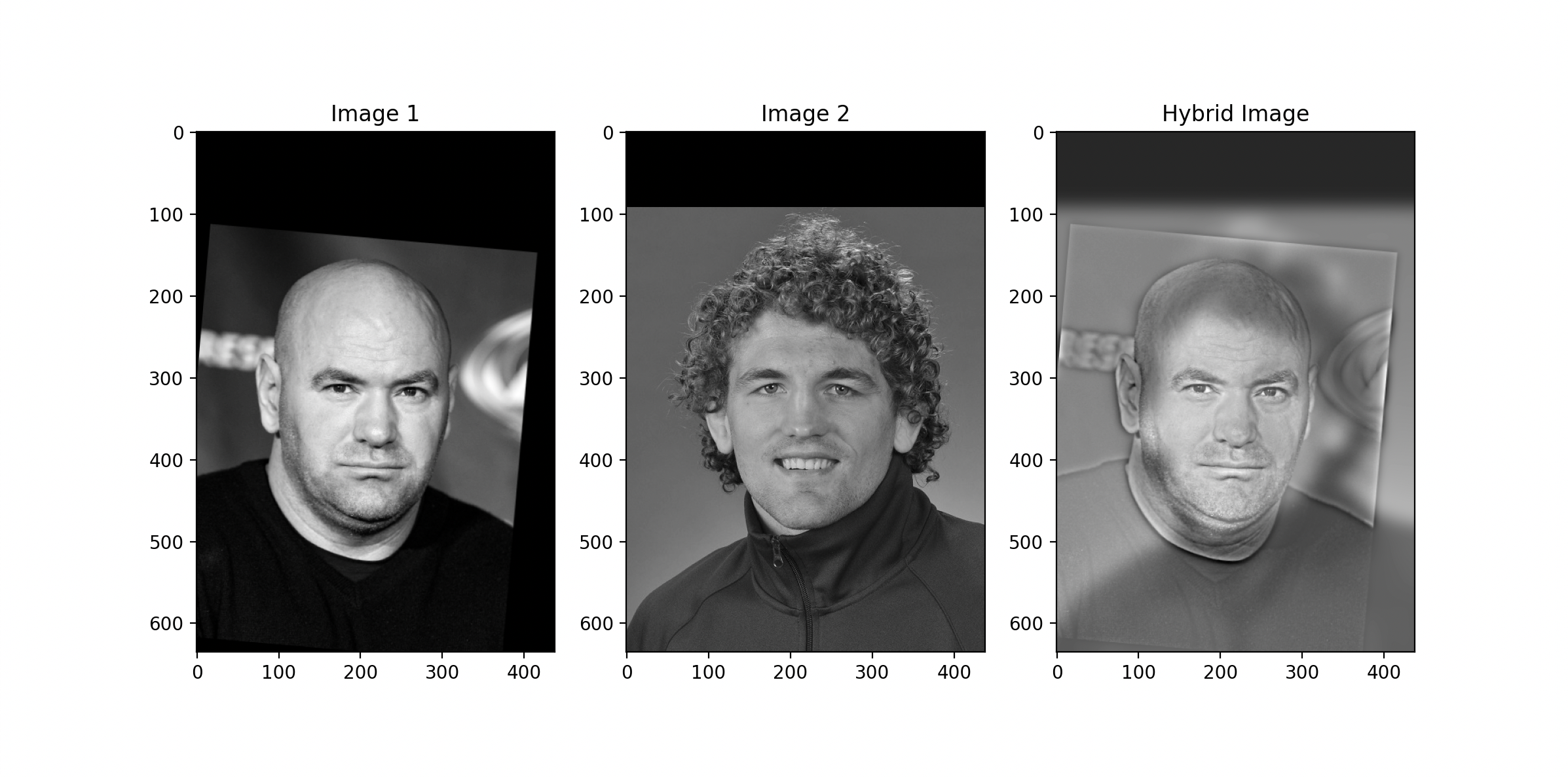
The Gaussian Filter acts a low pass filter as mentioned in the part above: image - gaussianfilter(image) will get the high frequencies of a picture. To get a hybrid image, we get the low frequencies from one image and combine it with the high frequencies of another image. The high frequencies will be visible at close distance, while the lower frequencies will dominate the picture at further distances since the human eye can't pick up on the high frequencies at large distances. I used the starter code to help align and rescale the images.

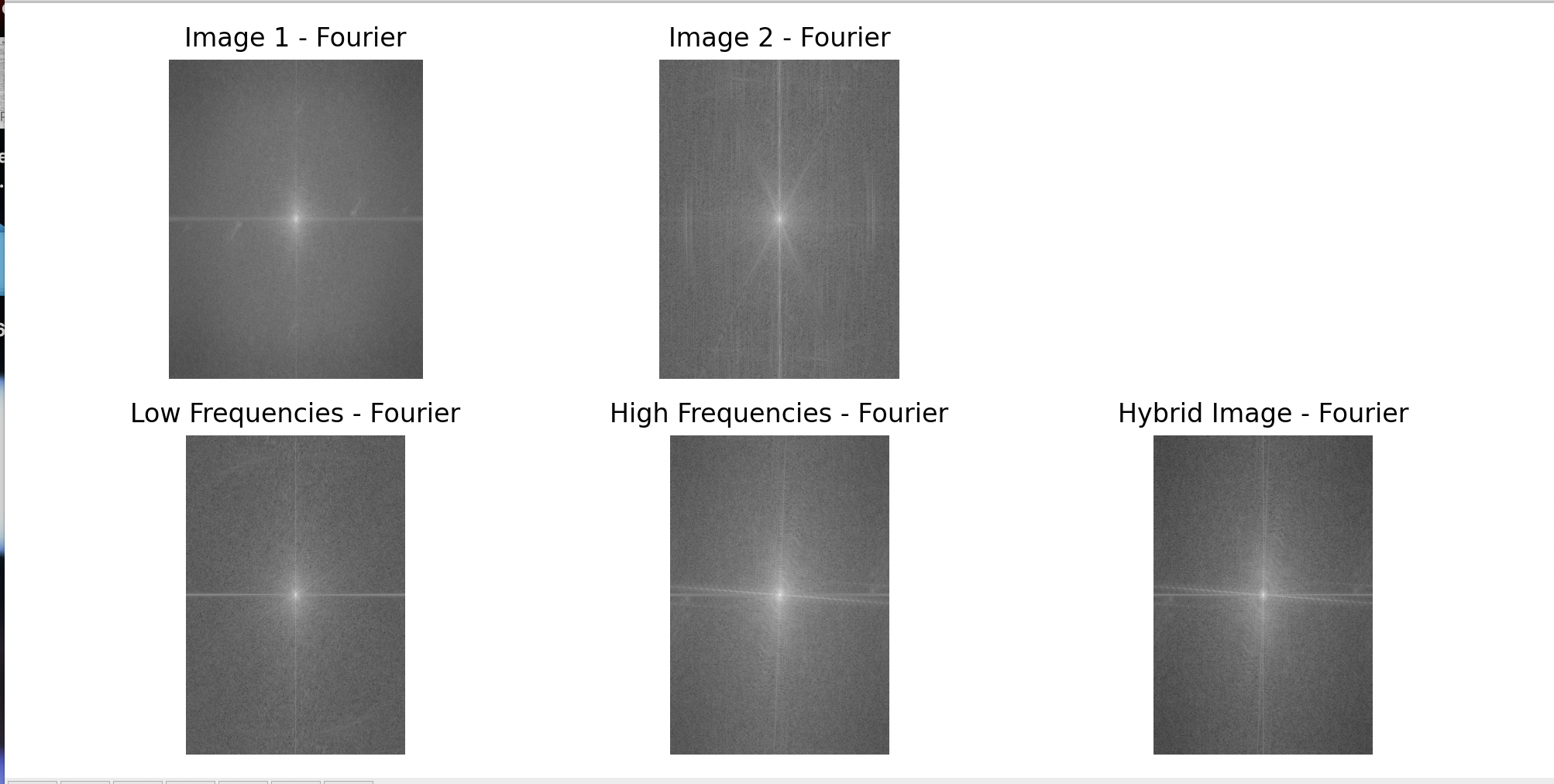
Here is the FFT of the images. As we can see the hybrid image just combines the low frequencies of one picture with the high frequencies of the other picture.

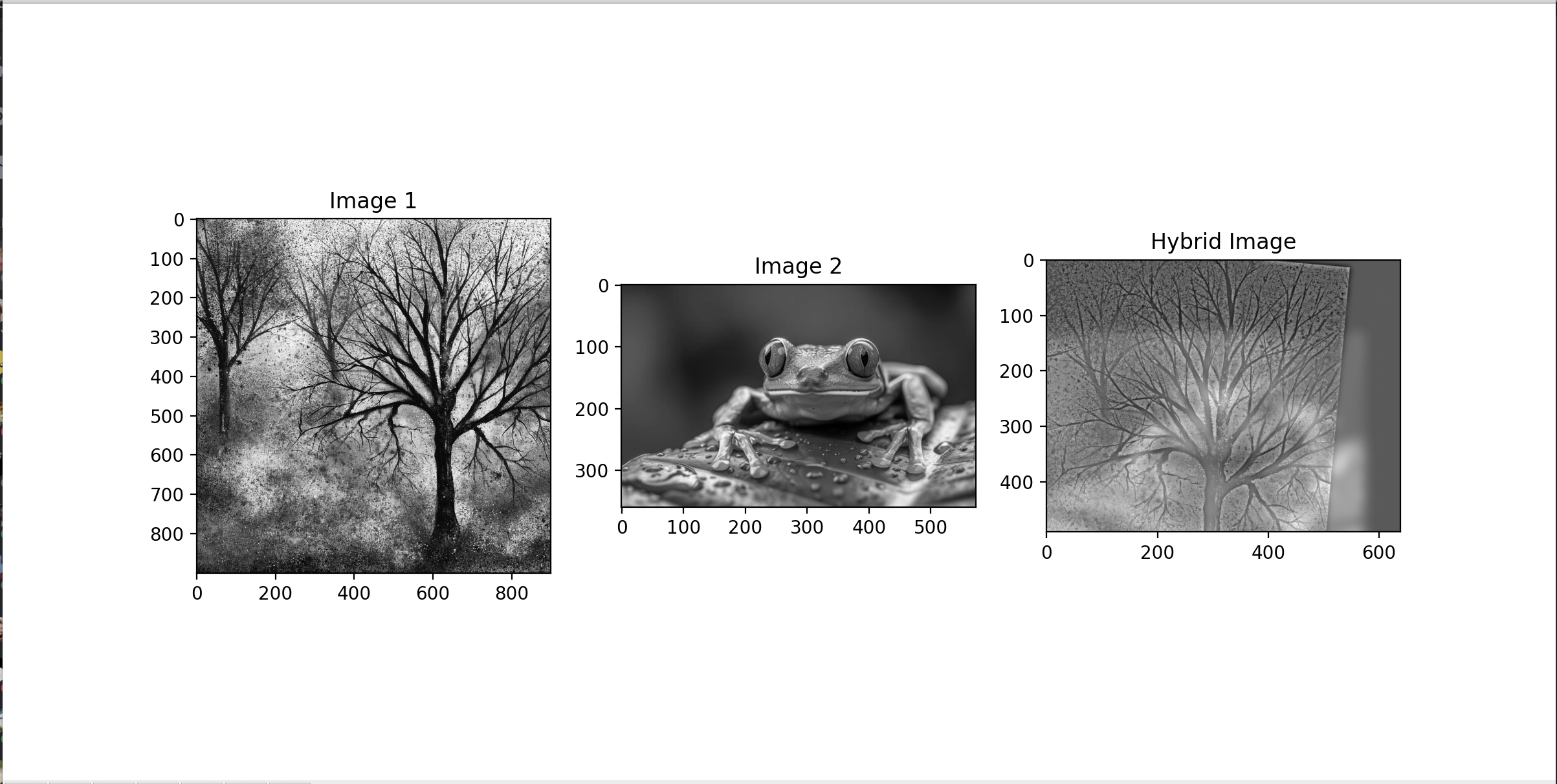
Below is our requirement for a failed an image. Why does this image fail? It's because they are both images with high frequencies due to the change in color and sharp details present. Even in a grayscale, it doesn't blend well because there's too many high frequencies present.

Part 2.3: Gaussian and Laplacian Stacks

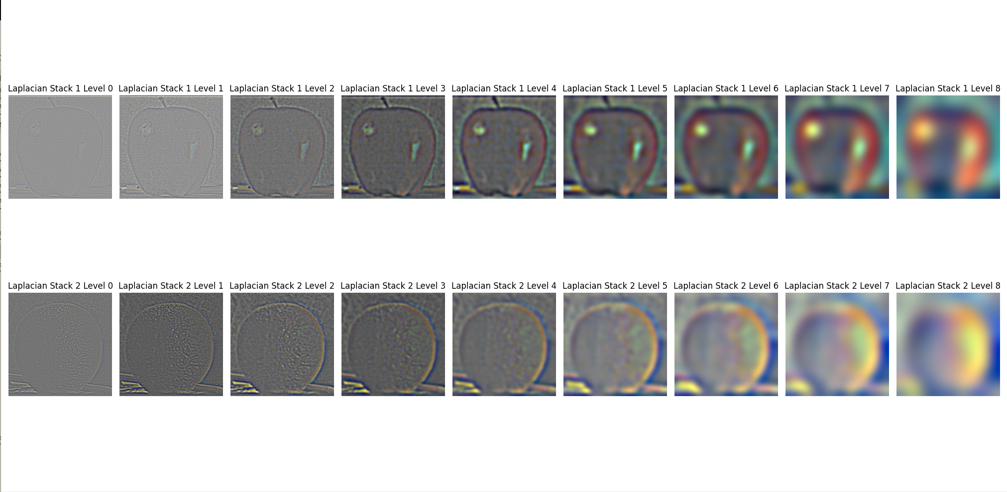
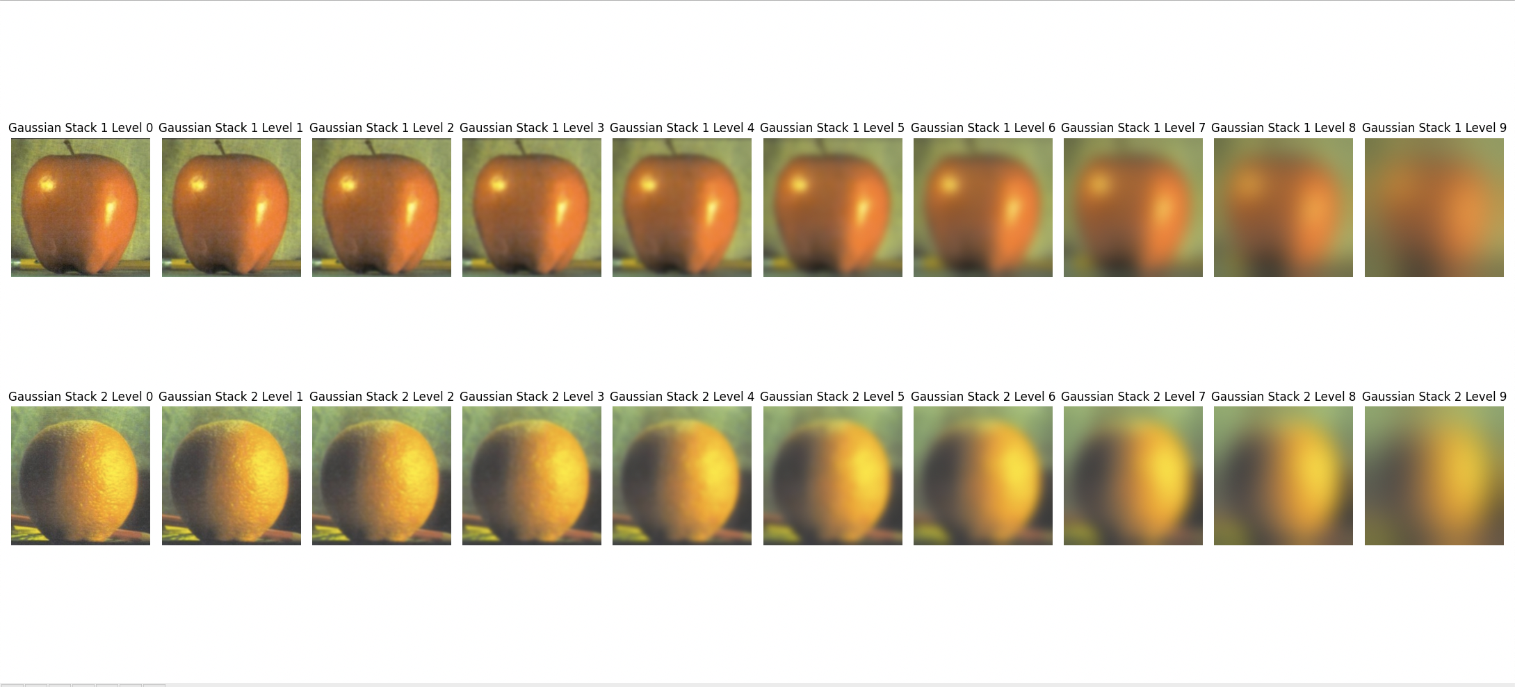
The Gaussian Stack is essentially the samething as the gaussian pyramid without random subsampling to downsize the image. All images in the stack are the same size, but the images are more progressively blurred. The Laplacian Stack is the difference between two consecutive layers in the gaussian stack. Initally, the difference between consecutive layers isn't much, but as we can see from the results, the difference becomes more noticable later down the laplacian stack. I put the results of both stacks for the apple and orange.

Part 2.4: Multiresolution Blending

The sum of the Laplacian Stack gets us the reconstrcuted image. Each layer is just the frequencies lost by each succesive gaussian filter applied. If we just use the vertical seam mask as is, we would get a sharp vertical seam. We can take advantage by getting the gaussian stack of the vertical seam mask. For each layer we use progressively more blurred versions in the gaussian stack of the vertical seam. So each layer becomes: blended = (gaussian_mask_stack[i] * laplacian_stack1[i]) + ((1 - gaussian_mask_stack[i]) * laplacian_stack2[i]). This helps transition to a much more smoother vertical seam. Now, we just add the blended laplacian stack to get the final image. The final product along with the recreation of the image in the paper is shown below.

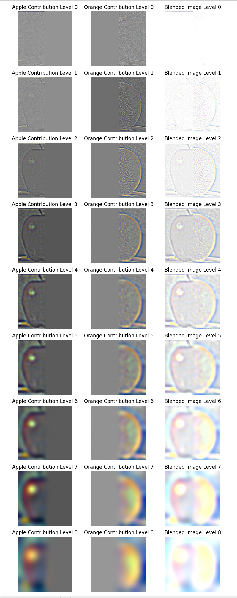
For our fun irregular mask, we used a circular mask to put LeBron's face on an apple. I imported some drawing tools to be able to draw the mask. To recreate this, you just need to run the program and draw the mask over LeBron's head (not just the boarder). Here is leApple.

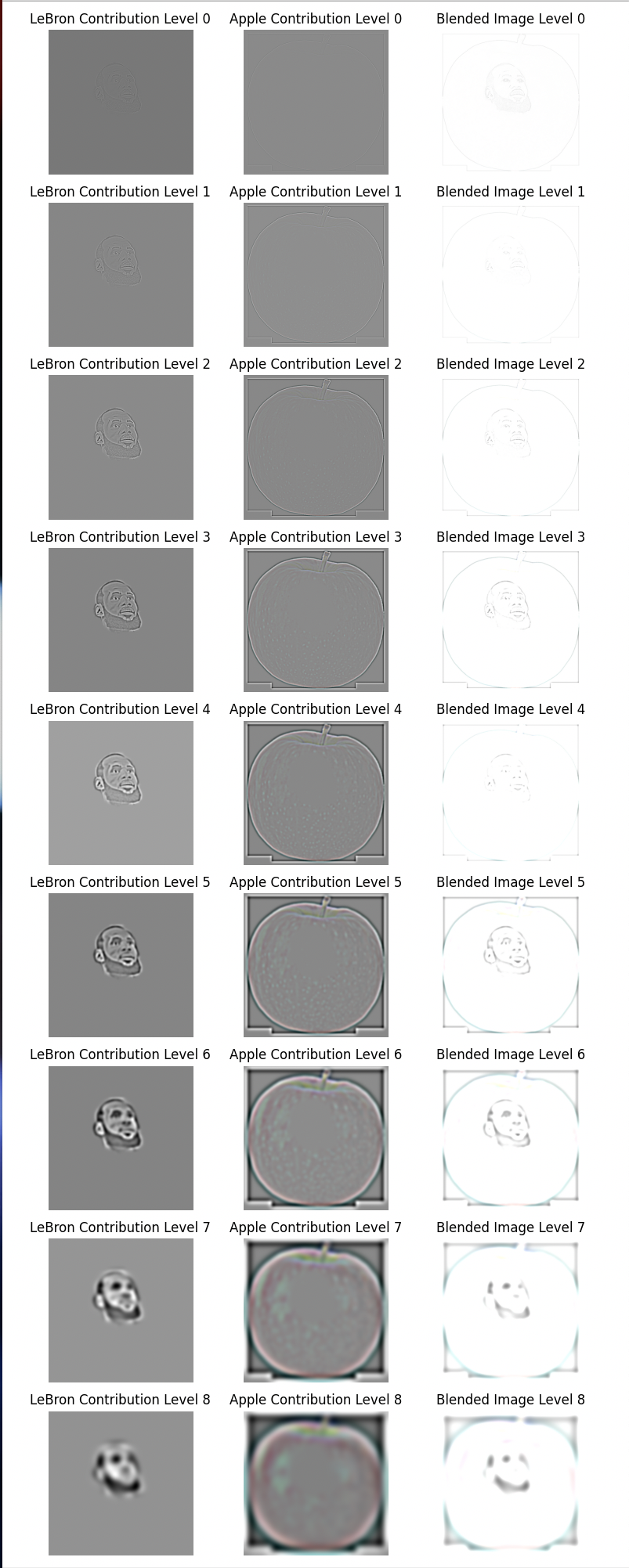
Here's a horizontal seam mask. Sorry the labeling on the title is off. I forgot to change the plot title names.

Conclusion

All of the requirements are above. For my most important thing I learned, I think it's how important the gaussian filter is. In every single part, I ended up using a gaussian filter. Even the laplacian stacks are derived from the gaussian filter. It shows how such a simple concept can be used to leverage power in image processing.